6. Local frequency analyses
[1]:
# Basic imports
import hvplot.xarray  # noqa
import numpy as np
import xarray as xr
import xdatasets

import xhydro as xh
import xhydro.frequency_analysis as xhfa
ERROR 1: PROJ: proj_create_from_database: Open of /home/docs/checkouts/readthedocs.org/user_builds/xhydro/conda/latest/share/proj failed
Redefining 'percent' (<class 'pint.delegates.txt_defparser.plain.UnitDefinition'>)
Redefining '%' (<class 'pint.delegates.txt_defparser.plain.UnitDefinition'>)
Redefining 'year' (<class 'pint.delegates.txt_defparser.plain.UnitDefinition'>)
Redefining 'yr' (<class 'pint.delegates.txt_defparser.plain.UnitDefinition'>)
Redefining 'C' (<class 'pint.delegates.txt_defparser.plain.UnitDefinition'>)
Redefining 'd' (<class 'pint.delegates.txt_defparser.plain.UnitDefinition'>)
Redefining 'h' (<class 'pint.delegates.txt_defparser.plain.UnitDefinition'>)
Redefining 'degrees_north' (<class 'pint.delegates.txt_defparser.plain.UnitDefinition'>)
Redefining 'degrees_east' (<class 'pint.delegates.txt_defparser.plain.UnitDefinition'>)
Redefining 'degrees' (<class 'pint.delegates.txt_defparser.plain.UnitDefinition'>)
Redefining '[speed]' (<class 'pint.delegates.txt_defparser.plain.DerivedDimensionDefinition'>)
/home/docs/checkouts/readthedocs.org/user_builds/xhydro/conda/latest/lib/python3.14/site-packages/xhydro/__init__.py:21: UserWarning: The `exactextract` library is not present in the environment and will not be used.
6.1. Data extraction and preparation
In this example, we will perform a frequency analysis using historical timeseries data collected from various sites. Our first step is to acquire a hydrological dataset. For this, we utilize the xdatasets library to retrieve hydrological data from the Ministère de l’Environnement, de la Lutte contre les changements climatiques, de la Faune et des
Parcs in Québec, Canada. Our query will focus on stations with IDs beginning with 020, and specifically those with natural flow pattern. Some stations have information on water levels, but will will only process streamflow data.
Alternatively, users can provide their own xarray.DataArray. When preparing the data for frequency analysis, it must adhere to the following requirements:
The dataset must include a
timedimension.If there is a 1D spatial dimension (e.g.,
idin the example below), it must contain an attributecf_rolewith the valuetimeseries_id.The variable must have at least a
unitsattribute. Although additional attributes, such aslong_nameandcell_methods, are not strictly required, they are expected byxclim, which is invoked during the frequency analysis. Missing these attributes will trigger warnings.
[2]:
ds = (
    xdatasets.Query(
        **{
            "datasets": {
                "deh": {
                    "id": ["020*"],
                    "regulated": ["Natural"],
                    "variables": ["streamflow"],
                }
            },
            "time": {"start": "1970-01-01", "minimum_duration": (15 * 365, "d")},
        }
    )
    .data.squeeze()
    .load()
)

# This dataset lacks some of the aforementioned attributes, so we need to add them.
ds = ds.rename({"streamflow": "q"})
ds["id"].attrs["cf_role"] = "timeseries_id"
ds["q"].attrs = {
    "long_name": "Streamflow",
    "units": "m3 s-1",
    "standard_name": "water_volume_transport_in_river_channel",
    "cell_methods": "time: mean",
}

# Clean some of the coordinates that are not needed for this example
ds = ds.drop_vars([c for c in ds.coords if c not in ["id", "time", "name"]])

# For the purpose of this example, we keep only 2 stations
ds = ds.isel(id=slice(3, 5))
ds
[2]:
<xarray.Dataset> Size: 327kB
Dimensions:  (id: 2, time: 20454)
Coordinates:
  * id       (id) object 16B '020602' '020802'
  * time     (time) datetime64[ns] 164kB 1970-01-01 1970-01-02 ... 2025-12-31
    name     (id) object 16B 'Dartmouth' 'Madeleine'
Data variables:
q (id, time) float32 164kB nan nan nan nan nan ... nan nan nan nan[3]:
ds.q.dropna("time", how="all").hvplot(
    x="time", grid=True, widget_location="bottom", groupby="id"
)
[3]:
6.2. Acquiring block maxima
The xhydro.indicators.get_yearly_op function can be used to extract block maxima from a time series. This function provides several options for customizing the extraction process, such as selecting the desired time periods and more. In the following section, we will present the main arguments available to help tailor the block maxima extraction to your needs.
[4]:
Help on function get_yearly_op in module xhydro.indicators.generic:

get_yearly_op(
    ds,
    op,
    *,
    input_var: str = 'q',
    window: int = 1,
    timeargs: dict | None = None,
    missing: str = 'skip',
    missing_options: dict | None = None,
    interpolate_na: bool = False
) -> xr.Dataset
    Compute yearly operations on a variable.

    Parameters
    ----------
    ds : xr.Dataset
        Dataset containing the variable to compute the operation on.
    op : str
        Operation to compute. One of ["max", "min", "mean", "sum"].
    input_var : str
        Name of the input variable. Defaults to "q".
    window : int
        Size of the rolling window. A "mean" operation is performed on the rolling window before the call to xclim.
        This parameter cannot be used with the "sum" operation.
    timeargs : dict, optional
        Dictionary of time arguments for the operation.
        Keys are the name of the period that will be added to the results (e.g. "winter", "summer", "annual").
        Values are up to two dictionaries, with both being optional.
        The first is {'freq': str}, where str is a frequency supported by xarray (e.g. "YS", "YS-JAN", "YS-DEC").
        It needs to be a yearly frequency. Defaults to "YS-JAN".
        The second is an indexer as supported by :py:func:`xclim.core.calendar.select_time`.
        Defaults to {}, which means the whole year.
        See :py:func:`xclim.core.calendar.select_time` for more information.
        Examples: {"winter": {"freq": "YS-DEC", "date_bounds": ["12-01", "02-28"]}}, {"jan": {"freq": "YS", "month": 1}}, {"annual": {}}.
    missing : str
        How to handle missing values. One of "skip", "any", "at_least_n", "pct", "wmo".
        See :py:func:`xclim.core.missing` for more information.
    missing_options : dict, optional
        Dictionary of options for the missing values' method. See :py:func:`xclim.core.missing` for more information.
    interpolate_na : bool
        Whether to interpolate missing values before computing the operation. Only used with the "sum" operation.
        Defaults to False.

    Returns
    -------
    xr.Dataset
        Dataset containing the computed operations, with one variable per indexer.
        The name of the variable follows the pattern `{input_var}{window}_{op}_{indexer}`.

    Notes
    -----
    If you want to perform a frequency analysis on a frequency that is finer than annual, simply use multiple timeargs
    (e.g. 1 per month) to create multiple distinct variables.
6.2.1. a) Defining seasons
Seasons can be defined using indexers compatible with xclim.core.calendar.select_time. Four types of indexers are currently supported:
month: A sequence of month numbers (e.g.,[1, 2, 12]for January, February, and December).season: A sequence of season abbreviations, with options being'DJF','MAM','JJA', and'SON'(representing Winter, Spring, Summer, and Fall, respectively).doy_bounds: A sequence specifying the inclusive bounds of the period in terms of day of year (e.g.,[152, 243]).date_bounds: Similar todoy_bounds, but using a month-day format ('%m-%d'), such as["01-15", "02-23"].
When using xhydro.indicators.get_yearly_op to calculate block maxima, the indexers should be grouped within a dictionary and passed to the timeargs argument. The dictionary keys should represent the requested period (e.g., 'winter', 'summer') and will be appended to the variable name. Each dictionary entry can include the following:
The indexer, as defined above (e.g.,
"date_bounds": ["02-11", "06-19"]).(Optional) An annual resampling frequency. This is mainly used for indexers that span across the year. For example, setting
"freq": "YS-DEC"will start the year in December instead of January.
[5]:
# Some examples
timeargs = {
    "spring": {"date_bounds": ["02-11", "06-19"]},
    "summer": {"doy_bounds": [152, 243]},
    "fall": {"month": [9, 10, 11]},
    "winter": {
        "season": ["DJF"],
        "freq": "YS-DEC",
    },  # To correctly wrap around the year, we need to specify the resampling frequency.
    "august": {"month": [8]},
    "annual": {},
}
6.2.2. b) Defining criteria for missing values
The xhydro.indicators.get_yearly_op function also includes two arguments, missing and missing_options, which allow you to define tolerances for missing data. These arguments leverage xclim to handle missing values, and the available options are detailed in the xclim documentation.
[6]:
import xclim

print(xclim.core.missing.__doc__)
Missing Values Identification
=============================

Indicators may use different criteria to determine whether a computed indicator value should be
considered missing. In some cases, the presence of any missing value in the input time series should result in a
missing indicator value for that period. In other cases, a minimum number of valid values or a percentage of missing
values should be enforced. The World Meteorological Organisation (WMO) suggests criteria based on the number of
consecutive and overall missing values per month.

`xclim` has a registry of missing value detection algorithms that can be extended by users to customize the behavior
of indicators. Once registered, algorithms can be used by setting the global option as
``xc.set_options(check_missing="method")`` or within indicators by setting the `missing` attribute of an
`Indicator` subclass. By default, `xclim` registers the following algorithms:

 * `any`: A result is missing if any input value is missing.
 * `some_but_not_all`: A result is missing if some but not all input values are missing.
 * `at_least_n`: A result is missing if less than a given number of valid values are present.
 * `pct`: A result is missing if more than a given fraction of its values are missing.
 * `wmo`: A result is missing if 11 days are missing, or 5 consecutive values are missing in a month.

To define another missing value algorithm, subclass :py:class:`MissingBase` and decorate it with
:py:func:`xclim.core.options.register_missing_method`. See subclassing guidelines in ``MissingBase``'s doc.
6.2.3. c) Simple example
Let’s start with a straightforward example using the timeargs dictionary defined earlier. In this case, we will set a tolerance where a maximum of 15% of missing data in a year will be considered acceptable for the year to be regarded as valid.
[7]:
ds_4fa = xh.indicators.get_yearly_op(
    ds, op="max", timeargs=timeargs, missing="pct", missing_options={"tolerance": 0.15}
)

ds_4fa
[7]:
<xarray.Dataset> Size: 3kB
Dimensions:       (id: 2, time: 56)
Coordinates:
  * id            (id) object 16B '020602' '020802'
  * time          (time) datetime64[ns] 448B 1970-01-01 ... 2025-01-01
    name          (id) object 16B 'Dartmouth' 'Madeleine'
Data variables:
    q_max_spring  (id, time) float32 448B nan 241.0 223.0 186.0 ... nan nan nan
    q_max_summer  (id, time) float32 448B nan 27.2 123.0 74.5 ... nan nan nan
    q_max_fall    (id, time) float32 448B nan 11.6 18.2 43.6 ... nan nan nan nan
    q_max_august  (id, time) float32 448B nan 12.1 21.9 12.2 ... nan nan nan nan
    q_max_annual  (id, time) float32 448B nan 241.0 223.0 186.0 ... nan nan nan
    q_max_winter  (id, time) float32 448B 8.5 5.52 3.48 48.1 ... nan nan nan nan
Attributes:
    cat:frequency:         yr
    cat:processing_level:  indicators
cat:id: [8]:
ds_4fa.q_max_summer.dropna("time", how="all").hvplot(
    x="time", grid=True, widget_location="bottom", groupby="id"
)
[8]:
6.2.4. d) Advanced example: Using custom seasons per year or per station
Customizing date ranges for each year or each station is not directly supported by xhydro.indicators.get_yearly_op. However, users can work around this limitation by masking their data before calling the function. When applying this approach, be sure to adjust the missing argument to accommodate the changes in the data availability.
In this example, we will define a season that starts on a random date in April and ends on a random date in June. Since we will mask almost the entire year, the tolerance for missing data should be adjusted accordingly. Instead of setting a general tolerance for missing data, we will use the at_least_n method to specify that at least 45 days of data must be available for the period to be considered valid.
[9]:
nyears = np.unique(ds.time.dt.year).size
dom_start = xr.DataArray(
    np.random.randint(1, 30, size=(nyears,)).astype("str"),
    dims=("year"),
    coords={"year": np.unique(ds.time.dt.year)},
)
dom_end = xr.DataArray(
    np.random.randint(1, 30, size=(nyears,)).astype("str"),
    dims=("year"),
    coords={"year": np.unique(ds.time.dt.year)},
)

mask = xr.zeros_like(ds["q"])
for y in dom_start.year.values:
    # Random mask of dates per year, between April and June.
    mask.loc[
        {
            "time": slice(
                str(y) + "-04-" + str(dom_start.sel(year=y).item()),
                str(y) + "-06-" + str(dom_end.sel(year=y).item()),
            )
        }
    ] = 1
[10]:
mask.hvplot(x="time", grid=True, widget_location="bottom", groupby="id")
[10]:
[11]:
# The name of the indexer will be used to identify the variable created here
timeargs_custom = {"custom": {}}

# We use .where() to mask the data that we want to ignore
masked = ds.where(mask == 1)
# Since we masked almost all the year, our tolerance for missing data should be changed accordingly
missing = "at_least_n"
missing_options = {"n": 45}

# We use xr.merge() to combine the results with the previous dataset.
ds_4fa = xr.merge(
    [
        ds_4fa,
        xh.indicators.get_yearly_op(
            masked,
            op="max",
            timeargs=timeargs_custom,
            missing=missing,
            missing_options=missing_options,
        ),
    ]
)
/tmp/ipykernel_4880/179792077.py:11: FutureWarning: In a future version of xarray the default value for compat will change from compat='no_conflicts' to compat='override'. This is likely to lead to different results when combining overlapping variables with the same name. To opt in to new defaults and get rid of these warnings now use `set_options(use_new_combine_kwarg_defaults=True) or set compat explicitly.
[12]:
ds_4fa.q_max_custom.dropna("time", how="all").hvplot(
    x="time", grid=True, widget_location="bottom", groupby="id"
)
[12]:
6.2.5. e) Alternative variable: Computing volumes
Frequency analysis can also be applied to volumes, following a similar workflow to that of streamflow data. The main difference is that if we’re starting with streamflow data, we must first convert it into volumes using xhydro.indicators.compute_volume (e.g., going from m3 s-1 to m3). Additionally, if necessary, the get_yearly_op function includes an argument, interpolate_na, which can be used to interpolate missing data before calculating the sum.
[13]:
# Get a daily volume from a daily streamflow
ds["volume"] = xh.indicators.compute_volume(ds["q"], out_units="hm3")

# We'll take slightly different indexers
timeargs_vol = {"spring": {"date_bounds": ["04-30", "06-15"]}, "annual": {}}

# The operation that we want here is the sum, not the max.
ds_4fa = xr.merge(
    [
        ds_4fa,
        xh.indicators.get_yearly_op(
            ds,
            op="sum",
            input_var="volume",
            timeargs=timeargs_vol,
            missing="pct",
            missing_options={"tolerance": 0.15},
            interpolate_na=True,
        ),
    ]
)
/tmp/ipykernel_4880/3886780519.py:8: FutureWarning: In a future version of xarray the default value for compat will change from compat='no_conflicts' to compat='override'. This is likely to lead to different results when combining overlapping variables with the same name. To opt in to new defaults and get rid of these warnings now use `set_options(use_new_combine_kwarg_defaults=True) or set compat explicitly.
[14]:
ds_4fa.volume_sum_spring.dropna("time", how="all").hvplot(
    x="time", grid=True, widget_location="bottom", groupby="id"
)
[14]:
6.3. Local frequency analysis
After extracting the raw data, such as annual maximums or minimums, the local frequency analysis is performed in three steps:
Use
xhydro.frequency_analysis.local.fitto determine the best set of parameters for a given number of statistical distributions.(Optional) Use
xhydro.frequency_analysis.local.criteriato compute goodness-of-fit criteria and assess how well each statistical distribution fits the data.Use
xhydro.frequency_analysis.local.parametric_quantilesto calculate return levels based on the fitted parameters.
To speed up the Notebook, we’ll only perform the analysis on a subset of variables.
[15]:
help(xhfa.local.fit)
Help on function fit in module xhydro.frequency_analysis.local:

fit(
    ds,
    *,
    distributions: list[str] | None = None,
    min_years: int | None = None,
    method: str = 'ML',
    periods: list[str] | list[list[str]] | None = None
) -> xr.Dataset
    Fit multiple distributions to data.

    Parameters
    ----------
    ds : xr.Dataset
        Dataset containing the data to fit. All variables will be fitted.
    distributions : list of str, optional
        List of distribution names as defined in `scipy.stats`. See https://docs.scipy.org/doc/scipy/reference/stats.html#continuous-distributions.
        Defaults to ["genextreme", "pearson3", "gumbel_r", "expon"].
    min_years : int, optional
        Minimum number of years required for a distribution to be fitted.
    method : str
        Fitting method. Defaults to "ML" (maximum likelihood).
    periods : list of str or list of list of str, optional
        Either [start, end] or list of [start, end] of periods to be considered.
        If multiple periods are given, the output will have a `horizon` dimension.
        If None, all data is used.

    Returns
    -------
    xr.Dataset
        Dataset containing the parameters of the fitted distributions, with a new dimension `scipy_dist` containing the distribution names.

    Notes
    -----
    In order to combine the parameters of multiple distributions, the size of the `dparams` dimension is set to the
    maximum number of unique parameters between the distributions.
The fit function enables the fitting of multiple statistical distributions simultaneously, such as ["genextreme", "pearson3", "gumbel_r", "expon"]. Since different distributions have varying parameter sets (and sometimes different naming conventions), xHydro handles this complexity by using a dparams dimension, filling in NaN values where needed. When the results interact with SciPy, such as the parametric_quantiles function, only the relevant parameters for each
distribution are passed. The selected distributions are stored in a newly created scipy_dist dimension.
[16]:
params = xhfa.local.fit(ds_4fa[["q_max_spring", "volume_sum_spring"]], min_years=15)

params
/home/docs/checkouts/readthedocs.org/user_builds/xhydro/conda/latest/lib/python3.14/site-packages/xhydro/frequency_analysis/local.py:93: FutureWarning: In a future version of xarray the default value for compat will change from compat='no_conflicts' to compat='override'. This is likely to lead to different results when combining overlapping variables with the same name. To opt in to new defaults and get rid of these warnings now use `set_options(use_new_combine_kwarg_defaults=True) or set compat explicitly.
[16]:
<xarray.Dataset> Size: 820B
Dimensions:            (scipy_dist: 4, id: 2, dparams: 4)
Coordinates:
  * scipy_dist         (scipy_dist) <U10 160B 'genextreme' ... 'expon'
  * id                 (id) object 16B '020602' '020802'
  * dparams            (dparams) <U5 80B 'c' 'skew' 'loc' 'scale'
    horizon            <U9 36B '1970-2025'
    name               (id) object 16B dask.array<chunksize=(2,), meta=np.ndarray>
Data variables:
    q_max_spring       (scipy_dist, id, dparams) float64 256B dask.array<chunksize=(1, 2, 4), meta=np.ndarray>
    volume_sum_spring  (scipy_dist, id, dparams) float64 256B dask.array<chunksize=(1, 2, 4), meta=np.ndarray>
Attributes:
    cat:frequency:         yr
    cat:processing_level:  indicators
cat:id: Criteria like AIC (Akaike Information Criterion), BIC (Bayesian Information Criterion), and AICC (Corrected AIC) are valuable tools for comparing the fit of different statistical models. These criteria balance the goodness-of-fit of a model with its complexity, helping to avoid overfitting. AIC and AICC are particularly useful when comparing models with different numbers of parameters, while BIC tends to penalize complexity more heavily, making it more conservative. Lower values of these criteria indicate better model performance, with AICC being especially helpful in small sample sizes. By using these metrics, we can objectively determine the most appropriate model for our data.
These three criteria can be accessed using xhydro.frequency_analysis.local.criteria. The results are added to a new criterion dimension. In this example, the AIC, BIC, and AICC all provide a weak indication that the Generalized Extreme Value (GEV) distribution is the best fit for the data, though the Gumbel distribution may also be a suitable choice. Conversely, the Pearson III failed to converge and the exponential distribution was rejected based on these criteria, suggesting that they
do not adequately fit the data.
[17]:
help(xhfa.local.criteria)
Help on function criteria in module xhydro.frequency_analysis.local:

criteria(ds: xr.Dataset, p: xr.Dataset) -> xr.Dataset
    Compute information criteria (AIC, BIC, AICC) from fitted distributions, using the log-likelihood.

    Parameters
    ----------
    ds : xr.Dataset
        Dataset containing the yearly data that was fitted.
    p : xr.Dataset
        Dataset containing the parameters of the fitted distributions.
        Must have a dimension `dparams` containing the parameter names and a dimension `scipy_dist` containing the distribution names.

    Returns
    -------
    xr.Dataset
        Dataset containing the information criteria for the distributions.
[18]:
criteria = xhfa.local.criteria(ds_4fa[["q_max_spring", "volume_sum_spring"]], params)

criteria["q_max_spring"].isel(id=0).compute()
[18]:
<xarray.DataArray 'q_max_spring' (scipy_dist: 4, criterion: 3)> Size: 96B
array([[596.59883519, 602.56578733, 597.07883519],
       [         inf,          inf,          inf],
       [595.61108485, 599.58905294, 595.84637896],
       [635.55247999, 639.53044808, 635.7877741 ]])
Coordinates:
  * scipy_dist  (scipy_dist) <U10 160B 'genextreme' 'pearson3' ... 'expon'
  * criterion   (criterion) <U4 48B 'aic' 'bic' 'aicc'
    id          <U6 24B '020602'
    name        object 8B 'Dartmouth'
    horizon     <U9 36B '1970-2025'
Attributes:
    original_long_name:      Maximum of variable
    original_units:          m3 s-1
    original_standard_name:  water_volume_transport_in_river_channel
    cell_methods:            time: mean
    history:                 [2026-07-06 20:54:27] fit: Estimate distribution...
    original_description:    Annual maximum of variable (02-11 to 06-19).
    long_name:               Information criteria
    description:             Information criteria for the distribution parame...
    scipy_dist:              ['genextreme', 'pearson3', 'gumbel_r', 'expon']
units: Finally, return periods can be obtained using xhfa.local.parametric_quantiles.
[19]:
Help on function parametric_quantiles in module xhydro.frequency_analysis.local:

parametric_quantiles(
    p: xr.Dataset,
    return_period: float | list[float],
    mode: str = 'max'
) -> xr.Dataset
    Compute quantiles from fitted distributions.

    Parameters
    ----------
    p : xr.Dataset
        Dataset containing the parameters of the fitted distributions.
        Must have a dimension `dparams` containing the parameter names and a dimension `scipy_dist` containing the distribution names.
    return_period : float or list of float
        Return period(s) in years.
    mode : {'max', 'min'}
        Whether the return period is the probability of exceedance (max) or non-exceedance (min).

    Returns
    -------
    xr.Dataset
        Dataset containing the quantiles of the distributions.
[20]:
rp = xhfa.local.parametric_quantiles(params, return_period=[2, 20, 100])

rp.load()
[20]:
<xarray.Dataset> Size: 660B
Dimensions:            (id: 2, scipy_dist: 4, return_period: 3)
Coordinates:
  * id                 (id) object 16B '020602' '020802'
  * scipy_dist         (scipy_dist) <U10 160B 'genextreme' ... 'expon'
  * return_period      (return_period) int64 24B 2 20 100
    horizon            <U9 36B '1970-2025'
    name               (id) object 16B 'Dartmouth' 'Madeleine'
    p_quantile         (return_period) float64 24B 0.5 0.95 0.99
Data variables:
    q_max_spring       (scipy_dist, return_period, id) float64 192B 185.5 ......
    volume_sum_spring  (scipy_dist, return_period, id) float64 192B 255.7 ......
Attributes:
    cat:frequency:         yr
    cat:processing_level:  indicators
cat:id: In a future release, plotting will be managed by a dedicated function. For now, we demonstrate the process using preliminary utilities in this notebook.
The function xhfa.local._prepare_plots generates the data points required to visualize the results of the frequency analysis. If log=True, it will return log-spaced x-values between xmin and xmax. Meanwhile, xhfa.local._get_plotting_positions calculates plotting positions for all variables in the dataset. It accepts alpha and beta arguments. For typical values, refer to the SciPy
documentation. By default, (0.4, 0.4) is used, which corresponds to the quantile unbiased method (Cunnane).
[21]:
data = xhfa.local._prepare_plots(params, xmin=1, xmax=1000, npoints=50, log=True)
pp = xhfa.local._get_plotting_positions(ds_4fa[["q_max_spring"]])
[22]:
# Plot the distributions
p1 = data.q_max_spring.hvplot(
    x="return_period", by="scipy_dist", grid=True, groupby=["id"], logx=True
)

# Plot the observations
p2 = pp.hvplot.scatter(
    x="q_max_spring_pp",
    y="q_max_spring",
    grid=True,
    groupby=["id"],
    logx=True,
)

# And now combining the plots
p1 * p2
[22]:
6.4. Uncertainties
Uncertainties are an important aspect of frequency analysis and should be considered when interpreting results. These uncertainties often stem from data quality, the choice of distribution, and the estimation of parameters. While visualizations can provide insights into the model fit, it’s crucial to quantify and account for uncertainties, such as confidence intervals for parameter estimates, to ensure robust conclusions.
In order to manage computational intensity, we will focus on a single catchment and limit the analysis to the two distributions that appeared to best fit the data.
[23]:
ds_4fa = ds_4fa.sel(id="020602")[["q_max_spring"]]
params = params.sel(id="020602", scipy_dist=["genextreme", "gumbel_r"])[
    ["q_max_spring"]
]
6.4.1. a) Bootstrapping the observations
One method for quantifying uncertainties is to bootstrap the observations. In this example, we will perform bootstrapping a small number of times to illustrate the process, though in practice, a higher number of iterations (e.g., 5000) is recommended to obtain more reliable estimates. Bootstrapping resamples the observed data with replacement to generate multiple datasets, which can then be used to assess the variability in the model’s parameters and results.
This can be accomplished by calling xhydro.frequency_analysis.uncertainties.bootstrap_obs.
[24]:
Help on function bootstrap_obs in module xhydro.frequency_analysis.uncertainties:

bootstrap_obs(obs: xr.DataArray, *, n_samples: int, seed: int | None = None) -> xr.DataArray
    Generate bootstrap samples from observed data.

    Parameters
    ----------
    obs : xarray.DataArray
        The observed data to bootstrap.
    n_samples : int
        The number of bootstrap samples to generate.
    seed : int, optional
        Seed for the random number generator.

    Returns
    -------
    xarray.DataArray
        Bootstrap samples with dimensions [samples, time].
[25]:
ds_4fa_boot_obs = xhfa.uncertainties.bootstrap_obs(ds_4fa, n_samples=35)
ds_4fa_boot_obs
[25]:
<xarray.Dataset> Size: 9kB
Dimensions:       (samples: 35, time: 56)
Coordinates:
  * samples       (samples) int64 280B 0 1 2 3 4 5 6 7 ... 28 29 30 31 32 33 34
  * time          (time) datetime64[ns] 448B 1970-01-01 ... 2025-01-01
    id            <U6 24B '020602'
    name          object 8B 'Dartmouth'
Data variables:
q_max_spring (samples, time) float32 8kB nan 184.0 64.97 ... 186.0 nanThis process will add a new dimension, samples, to the dataset. When used in conjunction with xhydro.frequency_analysis.local.fit, a new set of parameters will be computed for each sample. As a result, bootstrapping can become computationally expensive, especially as the number of bootstrap iterations increases.
[26]:
params_boot_obs = xhfa.local.fit(
    ds_4fa_boot_obs, distributions=["genextreme", "gumbel_r"]
)
rp_boot_obs = xhfa.local.parametric_quantiles(
    params_boot_obs, return_period=[2, 20, 100]
)
rp_boot_obs.load()
[26]:
<xarray.Dataset> Size: 2kB
Dimensions:        (samples: 35, scipy_dist: 2, return_period: 3)
Coordinates:
  * samples        (samples) int64 280B 0 1 2 3 4 5 6 7 ... 28 29 30 31 32 33 34
  * scipy_dist     (scipy_dist) <U10 80B 'genextreme' 'gumbel_r'
  * return_period  (return_period) int64 24B 2 20 100
    horizon        <U9 36B '1970-2025'
    id             <U6 24B '020602'
    name           object 8B 'Dartmouth'
    p_quantile     (return_period) float64 24B 0.5 0.95 0.99
Data variables:
q_max_spring (scipy_dist, return_period, samples) float64 2kB 185.1 ......6.4.2. b) Bootstrapping the distributions
In this approach, rather than resampling the observations directly, we resample the fitted distributions to estimate the uncertainty. This method allows us to assess the variability in the fitted distributions’ parameters. As with the previous example, we will perform a minimal number of bootstrap iterations to reduce computational load, but in practice, a higher number of iterations would provide more robust estimates of uncertainty.
This can be accomplished by calling xhydro.frequency_analysis.uncertainties.bootstrap_dist. Unlike bootstrap_obs, this method does not support lazy evaluation and requires a specific function for the fitting step: xhydro.frequency_analysis.uncertainties.fit_boot_dist.
[27]:
Help on function bootstrap_dist in module xhydro.frequency_analysis.uncertainties:

bootstrap_dist(ds_obs: xr.Dataset, ds_params: xr.Dataset, *, n_samples: int) -> xr.Dataset
    Generate bootstrap samples from a fitted distribution.

    Parameters
    ----------
    ds_obs : xarray.Dataset
        The observed data.
    ds_params : xarray.Dataset
        The fitted distribution parameters.
    n_samples : int
        The number of bootstrap samples to generate.

    Returns
    -------
    xarray.Dataset
        Bootstrap samples with dimensions [samples, time].

    Notes
    -----
    This function does not support lazy evaluation.
[28]:
Help on function fit_boot_dist in module xhydro.frequency_analysis.uncertainties:

fit_boot_dist(ds: xr.Dataset) -> xr.Dataset
    Fit distributions to bootstrap samples.

    Parameters
    ----------
    ds : xarray.Dataset
        The bootstrap samples to fit.

    Returns
    -------
    xarray.Dataset
        Fitted distribution parameters for each bootstrap sample.
[29]:
tmp_values = xhfa.uncertainties.bootstrap_dist(ds_4fa, params, n_samples=35)
params_boot_dist = xhfa.uncertainties.fit_boot_dist(tmp_values)
params_boot_dist
[29]:
<xarray.Dataset> Size: 2kB
Dimensions:       (scipy_dist: 2, samples: 35, dparams: 3)
Coordinates:
  * scipy_dist    (scipy_dist) <U10 80B 'genextreme' 'gumbel_r'
  * samples       (samples) int64 280B 0 1 2 3 4 5 6 7 ... 28 29 30 31 32 33 34
  * dparams       (dparams) <U5 60B 'c' 'loc' 'scale'
    horizon       <U9 36B '1970-2025'
    id            <U6 24B '020602'
    name          object 8B 'Dartmouth'
Data variables:
q_max_spring (scipy_dist, samples, dparams) float64 2kB dask.array<chunksize=(1, 35, 2), meta=np.ndarray>[30]:
rp_boot_dist = xhfa.local.parametric_quantiles(
    params_boot_dist.load(), return_period=[2, 20, 100]
)  # Lazy computing is not supported
rp_boot_dist
[30]:
<xarray.Dataset> Size: 2kB
Dimensions:        (samples: 35, scipy_dist: 2, return_period: 3)
Coordinates:
  * samples        (samples) int64 280B 0 1 2 3 4 5 6 7 ... 28 29 30 31 32 33 34
  * scipy_dist     (scipy_dist) <U10 80B 'genextreme' 'gumbel_r'
  * return_period  (return_period) int64 24B 2 20 100
    horizon        <U9 36B '1970-2025'
    id             <U6 24B '020602'
    name           object 8B 'Dartmouth'
    p_quantile     (return_period) float64 24B 0.5 0.95 0.99
Data variables: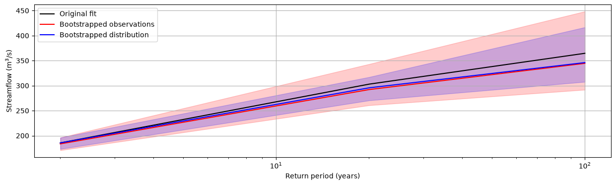
q_max_spring (scipy_dist, return_period, samples) float64 2kB 169.6 ......6.4.3. c) Comparison
Let’s show the difference between both approaches.
[31]:
import matplotlib.pyplot as plt

fig, ax = plt.subplots()
fig.set_figheight(4)
fig.set_figwidth(15)

# Subset the data
rp_orig = rp.q_max_spring.sel(id="020602", scipy_dist="genextreme")
boot_obs = rp_boot_obs.q_max_spring.sel(scipy_dist="genextreme")
boot_dist = rp_boot_dist.q_max_spring.sel(scipy_dist="genextreme")

# Original fit
ax.plot(
    rp_orig.return_period.values,
    rp_orig,
    "black",
    label="Original fit",
)

ax.plot(
    boot_obs.return_period.values,
    boot_obs.quantile(0.5, "samples"),
    "red",
    label="Bootstrapped observations",
)
boot_obs_05 = boot_obs.quantile(0.05, "samples")
boot_obs_95 = boot_obs.quantile(0.95, "samples")
ax.fill_between(
    boot_obs.return_period.values, boot_obs_05, boot_obs_95, alpha=0.2, color="red"
)

ax.plot(
    boot_dist.return_period.values,
    boot_dist.quantile(0.5, "samples"),
    "blue",
    label="Bootstrapped distribution",
)
boot_dist_05 = boot_dist.quantile(0.05, "samples")
boot_dist_95 = boot_dist.quantile(0.95, "samples")
ax.fill_between(
    boot_dist.return_period.values, boot_dist_05, boot_dist_95, alpha=0.2, color="blue"
)

plt.xscale("log")
plt.grid(visible=True)
plt.xlabel("Return period (years)")
plt.ylabel("Streamflow (m$^3$/s)")
ax.legend()
[31]:
<matplotlib.legend.Legend at 0x76e0137ca900>