5. Interpolation optimale¶

L’interpolation optimale est une méthode utilisée pour combiner des données spatialement distribuées (le « champ d’essai” ») avec des observations basées sur des points. Cette technique ajuste l’ensemble du champ en incorporant les écarts entre les données observées et le champ aux points d’observation, ce qui aboutit à un ajustement statistiquement optimal du champ d’essai. Par exemple, elle peut être utilisée pour fusionner les données de précipitation d’une réanalyse (comme ERA5) avec des données observées réelles, assurant que la précipitation de la réanalyse est corrigée sur l’ensemble du domaine.

Cette page montre comment utiliser xHydro pour réaliser une interpolation optimale pour la modélisation hydrologique en intégrant des simulations de type champ d’essai avec des observations. Dans ce cas, le champ d’essai est constitué des sorties d’un modèle hydrologique distribué, tandis que les observations correspondent à des mesures réelles aux stations hydrométriques. L’objectif est de corriger le champ d’essai (c’est-à-dire les sorties du modèle hydrologique) en utilisant des techniques d’interpolation optimale, selon l’approche décrite dans Lachance-Cloutier et al. (2017).

Lachance-Cloutier, S., Turcotte, R. and Cyr, J.F., 2017. Combining streamflow observations and hydrologic simulations for the retrospective estimation of daily streamflow for ungauged rivers in southern Quebec (Canada). Journal of hydrology, 550, pp.294-306.

L’interpolation optimale repose sur un ensemble d’hyperparamètres. Certains d’entre eux sont plus complexes que d’autres, alors décomposons les étapes principales.

La première étape consiste à calculer les différences (ou « écarts ») entre le débit observé et simulé aux stations où les deux valeurs sont disponibles. Ces différences doivent être mises à l’échelle en fonction de la surface du bassin versant pour s’assurer que les erreurs sont relatives et peuvent être correctement interpolées. De plus, nous prenons le logarithme de ces valeurs mises à l’échelle pour éviter les débits négatifs lors de l’extrapolation. Nous inverserons cette transformation plus tard dans le processus.

Ensuite, nous avons besoin de quelques informations supplémentaires, qui peuvent ou non être disponibles pour nos sites d’observation et de simulation. Cela inclut des estimations de :

La variance des observations aux sites jaugeables.
La variance des débits simulés aux sites d’observation.
La variance des débits simulés aux sites d’estimation, y compris ceux qui correspondent également à un site d’observation.

Ces valeurs peuvent être estimées dans des applications réelles en utilisant de longues séries temporelles de débits transformés logarithmiquement et mis à l’échelle, ou à partir des erreurs de mesure associées à l’instrumentation aux sites jaugeables. Ces paramètres peuvent également être ajustés en fonction de l’expérience passée ou par essais et erreurs.

La dernière composante dont nous avons besoin est la fonction de covariance d’erreur (ECF). En termes simples, l’interpolation optimale prend en compte la distance entre une observation (ou plusieurs observations) et le site où nous devons estimer une nouvelle valeur de débit. Intuitivement, une station de simulation proche d’une station d’observation devrait avoir une forte correlation avec celle-ci, tandis qu’une station plus éloignée aura une correlation plus faible. Par conséquent, nous avons besoin d’une fonction de covariance qui estime :

Le degré de covariabilité entre un point observé et un point simulé.
La distance entre ces points.

La fonction ECF est essentielle pour cela, et plusieurs modèles existent dans la littérature. Dans de nombreux cas, une forme de modèle sera choisie a priori, et ses paramètres seront ajustés pour mieux représenter la covariance entre les points.

Dans cet exemple de test, nous n’avons pas suffisamment de points ou de pas de temps pour développer un modèle (ou une paramétrisation) significatif à partir des données. En conséquence, nous allons imposer un modèle. xHydro inclut quatre modèles intégrés, où par[0] et par[1] sont les paramètres du modèle à calibrer (dans des circonstances normales), et h représente la distance entre les points :

Modèle 1:

\[\begin{flalign*} &\text{par}[0] \cdot \left( 1 + \frac{h}{\text{par}[1]} \right) \cdot \exp\left(- \frac{h}{\text{par}[1]} \right) && \text{— D'après Lachance-Cloutier et al. 2017.} \end{flalign*}\]
Modèle 2:

\[\begin{flalign*} &\text{par}[0] \cdot \exp\left( -0.5 \cdot \left( \frac{h}{\text{par}[1]} \right)^2 \right) && \end{flalign*}\]
Modèle 3:

\[\begin{flalign*} &\text{par}[0] \cdot \exp\left( -\frac{h}{\text{par}[1]} \right) && \end{flalign*}\]
Modèle 4:

\[\begin{flalign*} &\text{par}[0] \cdot \exp\left( -\frac{h^{\text{par}[1]}}{\text{par}[0]} \right) && \end{flalign*}\]

[1]:

import datetime as dt
from functools import partial
from pathlib import Path

import matplotlib.pyplot as plt
import numpy as np
import pandas as pd
import pooch
import xarray as xr
from scipy.stats import norm

import xhydro as xh
import xhydro.optimal_interpolation
from xhydro.testing.helpers import deveraux

ERROR 1: PROJ: proj_create_from_database: Open of /home/docs/checkouts/readthedocs.org/user_builds/xhydro-fr/conda/latest/share/proj failed
/home/docs/checkouts/readthedocs.org/user_builds/xhydro-fr/conda/latest/lib/python3.14/site-packages/xhydro/__init__.py:21: UserWarning: The `exactextract` library is not present in the environment and will not be used.

5.1. Exemple avec les données d’HYDROTEL¶

L’interpolation optimale repose sur les jeux de données observés et simulés et nécessite les informations suivantes :

Données observées pour les sites mesurés
Données simulées pour tous les sites
Aires de bassin (pour mettre à l’échelle les erreurs)
Latitude et longitude du bassin (pour développer le modèle d’erreur spatial)

Cet exemple utilisera un sous-ensemble de données générées à l’aide du modèle hydrologique HYDROTEL.

[2]:

# Get data
test_data_path = deveraux().fetch(
    "optimal_interpolation/OI_data_corrected.zip",
    pooch.Unzip(),
)
directory_to_extract_to = Path(test_data_path[0]).parent

# Read-in all the files and set to paths that we can access later.
qobs = xr.open_dataset(directory_to_extract_to / "A20_HYDOBS_TEST_corrected.nc").rename(
    {"streamflow": "q"}
)
qsim = xr.open_dataset(directory_to_extract_to / "A20_HYDREP_TEST_corrected.nc").rename(
    {"streamflow": "q"}
)
station_correspondence = xr.open_dataset(
    directory_to_extract_to / "station_correspondence.nc"
)
df_validation = pd.read_csv(
    directory_to_extract_to / "stations_retenues_validation_croisee.csv",
    dtype=str,
)
observation_stations = list(df_validation["No_station"])

Il y a trois jeux de données, ainsi qu’une liste :

qobs : Le jeu de données contenant les observations ponctuelles et les métadonnées des stations.
qsim : Le jeu de données contenant les simulations du champ d’essai (ici, les résultats bruts de HYDROTEL), y compris les métadonnées des stations simulées.
station_correspondence : Un jeu de données qui lie simplement les identifiants des stations entre les stations observées et simulées. Cela est nécessaire car les stations observées utilisent des identifiants « réels », tandis que les simulations distribuées utilisent souvent des identifiants codés ou numérotés séquentiellement.
observation_stations : Une liste des stations du jeu d’observations que nous voulons utiliser pour construire l’interpolation optimale.

[3]:

qobs

[4]:

qsim

[5]:

station_correspondence

[5]:

<xarray.Dataset> Size: 18kB
Dimensions:     (station: 296)
Dimensions without coordinates: station
Data variables:
    reach_id    (station) <U9 11kB ...
    station_id  (station) <U6 7kB ...

[6]:

print(
    f"There are a total of {len(observation_stations)} selected observation stations."
)
print(observation_stations)

There are a total of 96 selected observation stations.
['011508', '011509', '020602', '020802', '021601', '021915', '021916', '022003', '022301', '022601', '022704', '023303', '023401', '023402', '023702', '024003', '024007', '024010', '024014', '024015', '030101', '030103', '030215', '030234', '030282', '030335', '030345', '030424', '030425', '030905', '030907', '030919', '030921', '040129', '040204', '040841', '040830', '040840', '041902', '041903', '042103', '043012', '050144', '050135', '050304', '050408', '050409', '050702', '050801', '050812', '050915', '050916', '051001', '051005', '051006', '051301', '051502', '052228', '052231', '052601', '052606', '052805', '060101', '060102', '060202', '060601', '060704', '060901', '061020', '061022', '061024', '061028', '061307', '061502', '061801', '061901', '061905', '061909', '062102', '062114', '062701', '062803', '070401', '072301', '073502', '073503', '073801', '074701', '074902', '075702', '075705', '076201', '076601', '080101', '080106', '080707']

AVERTISSEMENT

Le module d’interpolation optimale dans xHydro est encore en développement et est fortement hard-codé, notamment en ce qui concerne les entrées. Attendez-vous à des changements significatifs à mesure que le code est refactorisé et amélioré.

Les jeux de données doivent respecter des exigences de formatage spécifiques.

Pour le jeu de données observées (qobs dans cet exemple), les conditions suivantes doivent être remplies :

Les dimensions doivent être station et time.
Les données de débit doivent être stockées dans une variable appelée streamflow.
L’aire de drainage du bassin doit être représentée dans une variable appelée drainage_area.
La latitude et la longitude des centroïdes du bassin doivent être stockées sous centroid_lat et centroid_lon (ce ne sont pas les coordonnées des stations hydrométriques).
Une variable appelée station_id doit exister, contenant un identifiant unique pour chaque station. Cela sera utilisé pour faire correspondre les stations d’observation avec leurs stations simulées correspondantes.

Pour le jeu de données simulées (qsim dans cet exemple), les exigences suivantes s’appliquent :

Les dimensions doivent être station et time.
Les données de débit doivent être dans une variable appelée streamflow.
L’aire” de drainage pour chaque bassin, telle que simulée par le modèle, doit être stockée dans une variable appelée drainage_area.
Les centroïdes des bassins doivent être représentés par les coordonnées lat et lon.
Une variable appelée station_id doit exister, contenant un identifiant unique pour chaque station simulée, utilisée pour la lier aux stations observées.

La table de correspondance (station_correspondence dans cet exemple) doit inclure :

station_id pour les stations observées.
reach_id pour les stations simulées.

L’interpolation optimale dans xHydro est principalement accessible via la fonction xhydro.optimal_interpolation.optimal_interpolation_fun.execute_interpolation. Lors de la validation croisée leave-one-out sur plusieurs bassins, l’ensemble du processus d’interpolation est répété pour chaque bassin. Dans chaque itération, une station d’observation est laissée de côté et gardée indépendante pour la validation. Ce processus peut être long, mais peut être parallélisé en ajustant le flag approprié et en définissant le nombre de cœurs CPU en fonction de la capacité de votre machine. Par défaut, le code n’utilise qu’un seul cœur, mais si vous choisissez d’en augmenter le nombre, le nombre maximal de cœurs utilisés sera limité à ([nombre-de-coeurs / 2] - 1) pour éviter de surcharger votre ordinateur.

[7]:

help(xhydro.optimal_interpolation.execute)

Help on function execute_interpolation in module xhydro.optimal_interpolation.optimal_interpolation_fun:

execute_interpolation(
qobs: xr.Dataset,
qsim: xr.Dataset,
station_correspondence: xr.Dataset,
observation_stations: list,
ratio_var_bg: float = 0.15,
percentiles: list[float] | None = None,
variogram_bins: int = 10,
parallelize: bool = False,
max_cores: int = 1,
leave_one_out_cv: bool = False,
form: int = 3,
hmax_divider: float = 2.0,
p1_bnds: list | None = None,
hmax_mult_range_bnds: list | None = None
) -> xr.Dataset
Run the interpolation algorithm for leave-one-out cross-validation or operational use.

Parameters
----------
qobs : xr.Dataset
Streamflow and catchment properties dataset for observed data.
qsim : xr.Dataset
Streamflow and catchment properties dataset for simulated data.
station_correspondence : xr.Dataset
Correspondence between the tag in the simulated files and the observed station number for the obs dataset.
observation_stations : list
Observed hydrometric dataset stations to be used in the ECF function building and optimal interpolation
application step.
ratio_var_bg : float
Ratio for background variance (default is 0.15).
percentiles : list(float), optional
List of percentiles to analyze (default is [25.0, 50.0, 75.0, 100.0]).
variogram_bins : int, optional
Number of bins to split the data to fit the semi-variogram for the ECF. Defaults to 10.
parallelize : bool
Execute the profiler in parallel or in series (default is False).
max_cores : int
Maximum number of cores to use for parallel processing.
leave_one_out_cv : bool
Flag to determine if the code should be run in leave-one-out cross-validation (True) or should be applied
operationally (False).
form : int
The form of the ECF equation to use (1, 2, 3 or 4. See documentation).
hmax_divider : float
Maximum distance for binning is set as hmax_divider times the maximum distance in the input data. Defaults to 2.
p1_bnds : list, optional
The lower and upper bounds of the parameters for the first parameter of the ECF equation for variogram fitting.
Defaults to [0.95, 1].
hmax_mult_range_bnds : list, optional
The lower and upper bounds of the parameters for the second parameter of the ECF equation for variogram fitting.
It is multiplied by "hmax", which is calculated to be the threshold limit for the variogram sill.
Defaults to [0.05, 3].

Returns
-------
xr.Dataset
An xarray dataset containing the flow quantiles and all the associated metadata.

[8]:

ds = xh.optimal_interpolation.execute(
    qobs=qobs.sel(time=slice("2018-11-01", "2019-01-01")),
    qsim=qsim.sel(time=slice("2018-11-01", "2019-01-01")),
    station_correspondence=station_correspondence,
    observation_stations=observation_stations,
    form=1,
    ratio_var_bg=0.15,
    percentiles=[25, 50, 75],
    parallelize=False,
    max_cores=1,
    leave_one_out_cv=False,
)

ds

Le jeu de données retourné contient une variable de débit appelée q avec les dimensions [percentile, station_id, time], fournissant des estimations pour tout percentile demandé afin d’évaluer l’incertitude. Explorons maintenant comment l’interpolation optimale a modifié le débit dans un bassin versant.

[9]:

# Get a pair of station ID at one of the stations used for optimal interpolation
pair = station_correspondence.where(
    station_correspondence.station_id == observation_stations[0], drop=True
)
obs_id = pair["station_id"].data
sim_id = pair["reach_id"].data

# Get the streamflow data
observed_flow_select = (
    qobs["q"]
    .where(qobs.station_id == obs_id, drop=True)
    .sel(time=slice("2018-11-01", "2019-01-01"))
    .squeeze()
)
raw_simulated_flow_select = (
    qsim["q"]
    .where(qsim.station_id == sim_id, drop=True)
    .sel(time=slice("2018-11-01", "2019-01-01"))
    .squeeze()
)
interpolated_flow_select = ds["q"].sel(
    station_id=sim_id[0], percentile=50.0, time=slice("2018-11-01", "2019-01-01")
)

[10]:

plt.plot(observed_flow_select, label="Observed flow")
plt.plot(raw_simulated_flow_select, label="Raw simulation")
plt.plot(interpolated_flow_select, label="Interpolated simulation")
plt.xlabel("Simulation day")
plt.ylabel("Streamflow (m³/s)")
plt.legend()
plt.show()

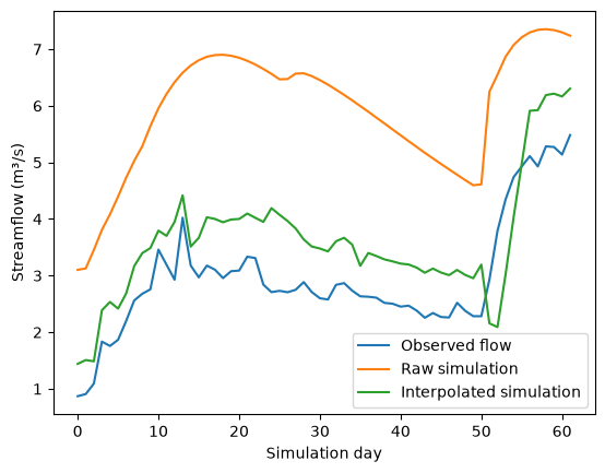
../_images/notebooks_optimal_interpolation_16_0.png

Nous pouvons observer que l’interpolation optimale a généralement aidé à rapprocher la simulation du modèle des données observées.