8. Extreme Value Analysis using Extremes.jl
This module provides an easy-to-use wrapper for the Extremes.jl Julia package, enabling seamless integration with xarray for extreme value analysis. However, do note that juliacall is not installed by default when installing xHydro. Consult the installation page for instructions.
The Extremes.jl package is specifically designed for analyzing extreme values and offers a variety of powerful features:
Block Maxima and Threshold Exceedance methods, including popular distributions such as
genextreme,gumbel_r, andgenpareto.Flexible parameter estimation techniques, supporting methods like
Probability-Weighted Moments (PWM),Maximum Likelihood Estimation (MLE), andBayesian Estimation.Compatibility with both stationary and non-stationary models for flexible modeling of future extreme events.
Return level estimation for quantifying the risk of extreme events over different return periods.
For further information on the Extremes.jl package, consult the following resources:
[1]:
import os

os.environ["PYTHON_JULIACALL_AUTOLOAD_IPYTHON_EXTENSION"] = (
    "no"  # To prevent random crashes with GitHub's testing interface
)

import matplotlib.pyplot as plt
import numpy as np
import pandas as pd
import pooch
from IPython.display import clear_output

import xhydro.extreme_value_analysis as xhe
from xhydro.testing.helpers import deveraux

clear_output(wait=False)
8.1. Data acquisition
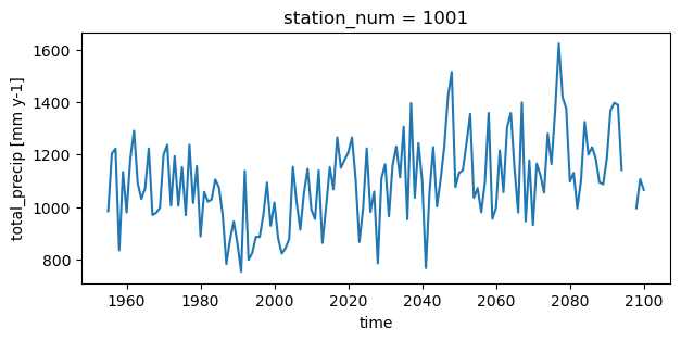
This example will use climate data from the GFDL-ESM4.1 model to demonstrate non-stationarity. The dataset includes annual total precipitation data from 1955 to 2100, spanning 97 virtual stations across the province of Quebec. For more information on how to access precipitation data or perform block maxima, consult the Local frequency analyses notebook.
[2]:
file = deveraux().fetch("extreme_value_analysis/NOAA_GFDL_ESM4.zip", pooch.Unzip())
[3]:
df = pd.read_csv(file[0], parse_dates=[0])[
    ["time", "station_num", "station_name", "total_precip"]
]
# That dataset is a CSV file, so we need to format it
ds = df.to_xarray()
ds = ds.set_coords(["time", "station_num", "station_name"])
ds = ds.set_index(index=["station_num", "time"])
ds = ds.unstack("index")
ds["total_precip"].attrs["units"] = "mm y-1"

# Take a subset for the example
ds = ds.isel(station_num=slice(0, 5))
ds
[3]:
<xarray.Dataset> Size: 13kB
Dimensions:       (station_num: 5, time: 146)
Coordinates:
  * station_num   (station_num) int64 40B 1001 1004 1008 1009 1012
  * time          (time) datetime64[ns] 1kB 1955-01-01 1956-01-01 ... 2100-01-01
    station_name  (station_num, time) object 6kB 'Dozois' ... 'Lac St-Francois'
Data variables:
total_precip (station_num, time) float64 6kB 983.6 1.204e+03 ... 1.065e+03[4]:
plt.figure(figsize=[7, 3])
ds.isel(station_num=0).total_precip.plot()
[4]:
[<matplotlib.lines.Line2D at 0x7fa05413bb30>]
WARNING
Currently, there is no way to provide Extremes.jl with a predefined set of parameters to directly calculate return levels. Until this functionality is implemented in either xHydro or Extremes.jl, the .fit() and .return_level() functions should be considered independent. Specifically, the .return_level() function will first estimate the distribution parameters before calculating the return levels.
8.2. Parameter estimation
The xhydro.extreme_value_analysis.fit function serves as the interface between xHydro and the Extremes.jl package. Most of the arguments mirror those used in the xhydro.frequency_analysis.local.fit function. The statistical distribution names have been made to align with those in SciPy. Below are a few key differences:
Bayesian Method (
BAYES): When using theBAYESmethod, you can specify two additional parameters:niter: Number of iterations for the Bayesian inference algorithm.warmup: Number of warmup iterations for the Bayesian inference.
Confidence Intervals: A significant addition to this function is the
confidence_levelparameter, which simplifies the process of obtaining confidence interval compared to the other options available inxHydro, as detailed in the other frequency analysis notebooks.
In this example, we will estimate a Generalized Extreme Value (GEV) distribution (genextreme) using the Probability Weighted Moments (PWM) method. Additionally, we will calculate and return the 95% confidence intervals for the estimated parameters.
[5]:
help(xhe.fit)
Help on function fit in module xhydro.extreme_value_analysis.parameterestimation:

fit(ds: 'xr.Dataset', locationcov: 'list[str] | None' = None, scalecov: 'list[str] | None' = None, shapecov: 'list[str] | None' = None, variables: 'list[str] | None' = None, dist: 'str | scipy.stats.rv_continuous' = 'genextreme', method: 'str' = 'ML', dim: 'str' = 'time', confidence_level: 'float' = 0.95, niter: 'int' = 5000, warmup: 'int' = 2000) -> 'xr.Dataset'
    Fit an array to a univariate distribution along a given dimension.

    Parameters
    ----------
    ds : xr.DataSet
        Xarray Dataset containing the data to be fitted.
    locationcov : list[str]
        List of names of the covariates for the location parameter.
    scalecov : list[str]
        List of names of the covariates for the scale parameter.
    shapecov : list[str]
        List of names of the covariates for the shape parameter.
    variables : list[str]
        List of variables to be fitted.
    dist : str or rv_continuous distribution object
        Name of the univariate distribution or the distribution object itself.
        Supported distributions are genextreme, gumbel_r, genpareto.
    method : {"ML", "PWM", "BAYES}
        Fitting method, either maximum likelihood (ML), probability weighted moments (PWM) or bayesian (BAYES).
    dim : str
        Specifies the dimension along which the fit will be performed (default: "time").
    confidence_level : float
        The confidence level for the confidence interval of each parameter.
    niter : int
        The number of iterations of the bayesian inference algorithm for parameter estimation (default: 5000).
    warmup : int
        The number of warmup iterations of the bayesian inference algorithm for parameter estimation (default: 2000).

    Returns
    -------
    xr.Dataset
        Dataset of fitted distribution parameters and confidence interval values.

    Notes
    -----
    Coordinates for which all values are NaNs will be dropped before fitting the distribution. If the array still
    contains NaNs or has less valid values than the number of parameters for that distribution,
    the distribution parameters will be returned as NaNs.
[6]:
fit_stationary = xhe.fit(
    ds,
    dist="genextreme",
    method="PWM",
    variables=["total_precip"],
    confidence_level=0.95,
)
fit_stationary
[6]:
<xarray.Dataset> Size: 460B
Dimensions:             (station_num: 5, dparams: 3)
Coordinates:
  * station_num         (station_num) int64 40B 1001 1004 1008 1009 1012
  * dparams             (dparams) <U5 60B 'shape' 'loc' 'scale'
Data variables:
    total_precip        (station_num, dparams) float64 120B 0.2012 ... 155.8
    total_precip_lower  (station_num, dparams) float64 120B 0.08579 ... 135.3
total_precip_upper (station_num, dparams) float64 120B 0.3243 ... 174.18.3. Return levels
As mentioned in the warning above, the xhydro.extreme_value_analysis.return_level function cannot accept pre-defined parameters and Extremes.jl must compute them internally. Therefore, with the inclusion of the return_period argument, all function parameters remain the same.
In this example, we will estimate a Gumbel distribution (gumbel_r) using the Maximum Likelihood (ML) method. Additionally, we will calculate and return the 95% confidence intervals for the estimated parameters.
[7]:
help(xhe.return_level)
Help on function return_level in module xhydro.extreme_value_analysis.parameterestimation:

return_level(ds: 'xr.Dataset', locationcov: 'list[str] | None' = None, scalecov: 'list[str] | None' = None, shapecov: 'list[str] | None' = None, variables: 'list[str] | None' = None, dist: 'str | scipy.stats.rv_continuous' = 'genextreme', method: 'str' = 'ML', dim: 'str' = 'time', confidence_level: 'float' = 0.95, return_period: 'float' = 100, niter: 'int' = 5000, warmup: 'int' = 2000, threshold_pareto: 'float | None' = None, nobs_pareto: 'int | None' = None, nobsperblock_pareto: 'int | None' = None) -> 'xr.Dataset'
    Compute the return level associated with a return period based on a given distribution.

    Parameters
    ----------
    ds : xr.DataSet
        Xarray Dataset containing the data for return level calculations.
    locationcov : list[str]
        List of names of the covariates for the location parameter.
    scalecov : list[str]
        List of names of the covariates for the scale parameter.
    shapecov : list[str]
        List of names of the covariates for the shape parameter.
    variables : list[str]
        List of variables to be fitted.
    dist : str or rv_continuous distribution object
        Name of the univariate distribution or the distribution object itself.
        Supported distributions are genextreme, gumbel_r, genpareto.
    method : {"ML", "PWM", "BAYES}
        Fitting method, either maximum likelihood (ML), probability weighted moments (PWM) or bayesian (BAYES).
    dim : str
        Specifies the dimension along which the fit will be performed (default: "time").
    confidence_level : float
        The confidence level for the confidence interval of each parameter.
    return_period : float
        Return period used to compute the return level.
    niter : int
        The number of iterations of the bayesian inference algorithm for parameter estimation (default: 5000).
    warmup : int
        The number of warmup iterations of the bayesian inference algorithm for parameter estimation (default: 2000).
    threshold_pareto : float
        The value above which the Pareto distribution is applied.
    nobs_pareto : int
        The total number of observations used when applying the Pareto distribution.
    nobsperblock_pareto : int
        The number of observations per block when applying the Pareto distribution.

    Returns
    -------
    xr.Dataset
        Dataset of with the return level and the confidence interval values.

    Notes
    -----
    Coordinates for which all values are NaNs will be dropped before fitting the distribution. If the array still
    contains NaNs or has less valid values than the number of parameters for that distribution,
    the distribution parameters will be returned as NaNs.
[8]:
rtnlv_stationary = xhe.return_level(
    ds,
    dist="gumbel_r",
    method="ML",
    variables=["total_precip"],
    confidence_level=0.95,
    return_period=100,
)
rtnlv_stationary
[8]:
<xarray.Dataset> Size: 168B
Dimensions:             (station_num: 5, return_period: 1)
Coordinates:
  * station_num         (station_num) int64 40B 1001 1004 1008 1009 1012
  * return_period       (return_period) int64 8B 100
Data variables:
    total_precip        (station_num, return_period) float64 40B 1.704e+03 .....
    total_precip_lower  (station_num, return_period) float64 40B 1.609e+03 .....
total_precip_upper (station_num, return_period) float64 40B 1.8e+03 ... ...8.4. Non-stationary model
So far, we’ve skipped three additional arguments—locationcov, scalecov, and shapecov—that accept variable names. These arguments allow you to introduce a non-linear aspect to the statistical model. In non-stationary models, explanatory variables (covariates) can be used to capture changes in model parameters over time or across different conditions. These covariates can represent factors such as time, geographic location, global temperature increases or CO2 concentrations, or any
other variable that may influence the distribution parameters.
Also, note that the PWM method cannot be used with non-stationary models.
For this example, we’ll keep it simple and assume that the location parameter varies as a linear function of the year. To do this, we’ll need to add a new variable containing the year to our dataset and then provide this variable to the locationcov argument.
[9]:
ds["year"] = ds.time.dt.year.broadcast_like(ds["total_precip"])
ds
[9]:
<xarray.Dataset> Size: 19kB
Dimensions:       (station_num: 5, time: 146)
Coordinates:
  * station_num   (station_num) int64 40B 1001 1004 1008 1009 1012
  * time          (time) datetime64[ns] 1kB 1955-01-01 1956-01-01 ... 2100-01-01
    station_name  (station_num, time) object 6kB 'Dozois' ... 'Lac St-Francois'
Data variables:
    total_precip  (station_num, time) float64 6kB 983.6 1.204e+03 ... 1.065e+03
year (station_num, time) int64 6kB 1955 1956 1957 ... 2099 2100In the case of the .fit() function, adding a covariate will introduce a new entry under the dparams dimension. For this example, it created a new entry called loc_year_covariate under the dparams dimension.
[10]:
fit_non_stationary = xhe.fit(
    ds,
    dist="genextreme",
    method="ML",
    variables=["total_precip"],
    locationcov=["year"],
    confidence_level=0.95,
)
fit_non_stationary
[10]:
<xarray.Dataset> Size: 808B
Dimensions:             (station_num: 5, dparams: 4)
Coordinates:
  * station_num         (station_num) int64 40B 1001 1004 1008 1009 1012
  * dparams             (dparams) <U18 288B 'shape' 'loc' ... 'scale'
Data variables:
    total_precip        (station_num, dparams) float64 160B 0.2051 ... 144.3
    total_precip_lower  (station_num, dparams) float64 160B 0.1022 ... 127.0
total_precip_upper (station_num, dparams) float64 160B 0.308 ... 164.0In the case of the .return_level() function, adding a covariate preserves the original dimensions, including the dimension along which the return_level is computed (e.g., time ).
[11]:
rtnlv_non_stationary = xhe.return_level(
    ds,
    dist="gumbel_r",
    method="ML",
    dim="time",
    variables=["total_precip"],
    locationcov=["year"],
    confidence_level=0.95,
    return_period=100,
)

rtnlv_non_stationary
[11]:
<xarray.Dataset> Size: 25kB
Dimensions:             (station_num: 5, time: 146, return_period: 1)
Coordinates:
  * station_num         (station_num) int64 40B 1001 1004 1008 1009 1012
  * time                (time) datetime64[ns] 1kB 1955-01-01 ... 2100-01-01
    station_name        (station_num, time) object 6kB 'Dozois' ... 'Lac St-F...
  * return_period       (return_period) int64 8B 100
Data variables:
    total_precip        (station_num, time) float64 6kB 1.557e+03 ... 1.771e+03
    total_precip_lower  (station_num, time) float64 6kB 1.457e+03 ... 1.672e+03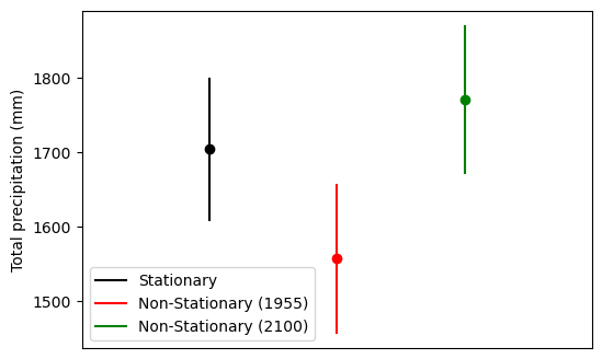
total_precip_upper (station_num, time) float64 6kB 1.656e+03 ... 1.87e+038.4.1. Comparison of the return level using the stationary and non-stationary model
[12]:
import matplotlib.pyplot as plt
import numpy as np

fig, ax = plt.subplots()
fig.set_figheight(4)
fig.set_figwidth(6)

# Stationary fit
plt.plot(
    np.array([1, 1]),
    np.array(
        [
            rtnlv_stationary.total_precip_lower.isel(station_num=0),
            rtnlv_stationary.total_precip_upper.isel(station_num=0),
        ]
    ),
    "black",
    label="Stationary",
)
plt.scatter(
    np.array([1]),
    np.array([rtnlv_stationary.total_precip.isel(station_num=0)]),
    c="black",
)

plt.plot(
    np.array([2, 2]),
    np.array(
        [
            rtnlv_non_stationary.total_precip_lower.isel(station_num=0, time=0),
            rtnlv_non_stationary.total_precip_upper.isel(station_num=0, time=0),
        ]
    ),
    "red",
    label="Non-Stationary (1955)",
)
plt.scatter(
    np.array([2]),
    np.array([rtnlv_non_stationary.total_precip.isel(station_num=0, time=0)]),
    c="red",
)

plt.plot(
    np.array([3, 3]),
    np.array(
        [
            rtnlv_non_stationary.total_precip_lower.isel(station_num=0, time=-1),
            rtnlv_non_stationary.total_precip_upper.isel(station_num=0, time=-1),
        ]
    ),
    "green",
    label="Non-Stationary (2100)",
)
plt.scatter(
    np.array([3]),
    np.array([rtnlv_non_stationary.total_precip.isel(station_num=0, time=-1)]),
    c="green",
)

plt.xlim([0, 4])
plt.xticks([])
plt.ylabel("Total precipitation (mm)")
ax.legend()
[12]:
<matplotlib.legend.Legend at 0x7f9f63a61340>
8.5. Working with dask.array Chunks
Currently, the Python-to-Julia interaction is not thread-safe. To mitigate potential issues, it is recommended to use the dask.scheduler="processes" option when computing results. This ensures that tasks are executed in separate Python processes, providing better isolation and avoiding thread-related conflicts.
[ ]:
ds_c = ds.chunk({"time": -1, "station_num": 1})

fit_stationary_c = xhe.fit(
    ds_c,
    dist="genextreme",
    method="ml",
    variables=["total_precip"],
    confidence_level=0.95,
)
fit_stationary_c = fit_stationary_c.compute(scheduler="processes")
clear_output(wait=False)
[14]:
fit_stationary_c
[14]:
<xarray.Dataset> Size: 460B
Dimensions:             (station_num: 5, dparams: 3)
Coordinates:
  * station_num         (station_num) int64 40B 1001 1004 1008 1009 1012
  * dparams             (dparams) <U5 60B 'shape' 'loc' 'scale'
Data variables:
    total_precip        (station_num, dparams) float64 120B dask.array<chunksize=(1, 3), meta=np.ndarray>
    total_precip_lower  (station_num, dparams) float64 120B dask.array<chunksize=(1, 3), meta=np.ndarray>
    total_precip_upper  (station_num, dparams) float64 120B dask.array<chunksize=(1, 3), meta=np.ndarray>