10. Climate change analysis of hydrological data
[1]:
# Imports
from pathlib import Path

import hvplot.xarray  # noqa
import numpy as np
import pooch
import xarray as xr
import xclim

import xhydro as xh
from xhydro.testing.helpers import deveraux

D = deveraux()

# Future streamflow file (1 file - Hydrotel driven by BCC-CSM-1.1(m))
streamflow_file = D.fetch("cc_indicators/streamflow_BCC-CSM1.1-m_rcp45.nc")

# Reference mean annual streamflow (QMOYAN) for 6 calibrations of Hydrotel
reference_files = D.fetch("cc_indicators/reference.zip", pooch.Unzip())

# Future deltas of QMOYAN (63 simulations x 6 calibrations of Hydrotel)
deltas_files = D.fetch("cc_indicators/deltas.zip", pooch.Unzip())
ERROR 1: PROJ: proj_create_from_database: Open of /home/docs/checkouts/readthedocs.org/user_builds/xhydro/conda/stable/share/proj failed
/home/docs/checkouts/readthedocs.org/user_builds/xhydro/conda/stable/lib/python3.14/site-packages/xhydro/__init__.py:21: UserWarning: The `exactextract` library is not present in the environment and will not be used.
While there is a vast array of analyses that can be performed to assess the impacts of climate change on hydrology, this notebook covers some of the most common steps:
Computing a list of relevant indicators over climatological periods.
Computing future differences to assess the changes.
Computing ensemble statistics to evaluate future changes and variability.
INFO
Several functions from the xscen library have been integrated into xhydro to simplify access for users, such as those in xhydro.indicators and xhydro.cc. This notebook will cover the basics, but for further details on these functions, please refer to the following resources:
10.1. Computing hydrological indicators over a given time period
Hydrological indicators can be categorized into two main types:
Frequential indicators: These indicators describe hydrological events that occur at recurring intervals. They include metrics like the maximum 20-year flow (
Qmax20) or the minimum 2-year 7-day average flow in summer (Q7min2_summer). The methodology for computing these indicators is covered in the Local Frequency Analysis notebook.Non-frequential indicators: These indicators do not explicitly describe recurrence, but rather absolute values or trends in hydrological variables. They include metrics like average yearly flow.
Since frequential indicators are already covered in another example, this notebook will focus on the methodology for computing non-frequential indicators using xhydro.indicators.compute_indicators. This function is built on top of xclim and supports both predefined indicators, such as xclim.indicator.land.doy_qmax, as well as custom indicators created using xclim.core.indicator.Indicator.from_dict. The latter option can be quite complex—see the box below for more information. For
advanced users, indicator construction can also be defined through a YAML file.
The output of xhydro.indicators.compute_indicators is a dictionary, where each key represents the frequency of the requested indicators, following the pandas nomenclature. In our example, we will only use yearly data starting in January, so the frequency will be YS-JAN.
INFO
Custom indicators in xHydro are built by following the YAML formatting required by xclim.
A custom indicator built using xclim.core.indicator.Indicator.from_dict will need these elements:
“data”: A dictionary with the following information:
“base”: The “YAML ID” obtained from here.
“input”: A dictionary linking the default xclim input to the name of your variable. Needed only if it is different. In the link above, they are the string following “Uses:”.
“parameters”: A dictionary containing all other parameters for a given indicator. In the link above, the easiest way to access them is by clicking the link in the top-right corner of the box describing a given indicator.
More entries can be used here, as described in the xclim documentation under “identifier”.
“identifier”: A custom name for your indicator. This will be the name returned in the results.
“module”: Needed, but can be anything. To prevent an accidental overwriting of
xclimindicators, it is best to use something different from: [“atmos”, “land”, “generic”].
The example file used in this notebook is a daily time series of streamflow data, generated from the HYDROTEL hydrological model. This data is driven by bias-adjusted outputs from the BCC-CSM-1.1(m) climatological model (RCP4.5), spanning the years 1950 to 2100. For this example, the dataset includes data from just 2 stations. The function xhydro.indicators.compute_indicators can be used with any number of indicators. For this example, we will compute the mean annual flow and the mean
summer-fall flow.
[2]:
ds = xr.open_dataset(streamflow_file).rename({"streamflow": "q"})
ds.q.hvplot(x="time", grid=True, widget_location="bottom", groupby="station")
[2]:
[3]:
Help on function compute_indicators in module xscen.indicators:

compute_indicators(
    ds: xr.Dataset,
    indicators: str | os.PathLike | Sequence[Indicator] | Sequence[tuple[str, Indicator]] | ModuleType,
    *,
    periods: list[str] | list[list[str]] | None = None,
    restrict_years: bool = True,
    to_level: str | None = 'indicators',
    rechunk_input: bool = False
) -> dict
    Calculate variables and indicators based on a YAML call to xclim.

    The function cuts the output to be the same years as the inputs.
    Hence, if an indicator creates a timestep outside the original year range (e.g. the first DJF for QS-DEC),
    it will not appear in the output.

    Parameters
    ----------
    ds : xr.Dataset
        Dataset to use for the indicators.
    indicators : str or os.PathLike or Sequence[Indicator] or Sequence[tuple[str, Indicator]] or ModuleType
        Path to a YAML file that instructs on how to calculate missing variables.
        Can also be only the "stem", if translations and custom indices are implemented.
        Can be the indicator module directly, or a sequence of indicators or a sequence of
        tuples (indicator name, indicator) as returned by `iter_indicators()`.
    periods : list of str or list of lists of str, optional
        Either [start, end] or list of [start, end] of continuous periods over which to compute the indicators.
        This is needed when the time axis of ds contains some jumps in time.
        If None, the dataset will be considered continuous.
    restrict_years : bool
        If True, cut the time axis to be within the same years as the input.
        This is mostly useful for frequencies that do not start in January, such as QS-DEC.
        In that instance, `xclim` would start on previous_year-12-01 (DJF), with a NaN.
        `restrict_years` will cut that first timestep. This should have no effect on YS and MS indicators.
    to_level : str, optional
        The processing level to assign to the output.
        If None, the processing level of the inputs is preserved.
    rechunk_input : bool
        If True, the dataset is rechunked with :py:func:`flox.xarray.rechunk_for_blockwise`
        according to the resampling frequency of the indicator. Each rechunking is done
        once per frequency with :py:func:`xscen.utils.rechunk_for_resample`.

    Returns
    -------
    dict
        Dictionary (keys = timedeltas) with indicators separated by temporal resolution.

    See Also
    --------
    xclim.indicators : Indicators module of xclim.
    xclim.core.indicator.build_indicator_module_from_yaml : YAML indicator constructor function of xclim.
[4]:
Help on method from_dict in module xclim.core.indicator:

from_dict(data: dict, identifier: str, module: str | None = None) -> Indicator class method of xclim.core.indicator.Indicator
    Create an indicator subclass and instance from a dictionary of parameters.

    Most parameters are passed directly as keyword arguments to the class constructor, except:

    - "base" : A subclass of Indicator or a name of one listed in
      :py:data:`xclim.core.indicator.registry` or
      :py:data:`xclim.core.indicator.base_registry`. When passed, it acts as if
      `from_dict` was called on that class instead.
    - "compute" : A string function name translates to a
      :py:mod:`xclim.indices.generic` or :py:mod:`xclim.indices` function.

    Parameters
    ----------
    data : dict
        The exact structure of this dictionary is detailed in the submodule documentation.
    identifier : str
        The name of the subclass and internal indicator name.
    module : str
        The module name of the indicator. This is meant to be used only if the indicator
        is part of a dynamically generated submodule, to override the module of the base class.

    Returns
    -------
    Indicator
        A new Indicator instance.
[5]:
indicators = [
    # 1st indicator: Mean annual flow
    xclim.core.indicator.Indicator.from_dict(
        data={
            "base": "stats",
            "input": {"da": "q"},
            "parameters": {"op": "mean"},
        },
        identifier="QMOYAN",
        module="hydro",
    ),
    # 2nd indicator: Mean summer-fall flow
    xclim.core.indicator.Indicator.from_dict(
        data={
            "base": "stats",
            "input": {"da": "q"},
            "parameters": {"op": "mean", "indexer": {"month": [6, 7, 8, 9, 10, 11]}},
        },  # The indexer is used to restrict available data to the relevant months only
        identifier="QMOYEA",
        module="hydro",
    ),
]

# Call compute_indicators
dict_indicators = xh.indicators.compute_indicators(ds, indicators=indicators)

dict_indicators
[5]:
{'YS-JAN': <xarray.Dataset> Size: 4kB
 Dimensions:        (station: 2, time: 151)
 Coordinates:
   * station        (station) <U9 72B 'ABIT00057' 'ABIT00058'
   * time           (time) datetime64[ns] 1kB 1950-01-01 ... 2100-01-01
     lat            (station) float32 8B ...
     lon            (station) float32 8B ...
     drainage_area  (station) float32 8B ...
 Data variables:
     QMOYAN         (station, time) float32 1kB nan nan nan ... 0.8027 0.743 nan
     QMOYEA         (station, time) float32 1kB nan nan nan ... 0.385 1.035
 Attributes: (12/48)
     institution:                    DEH (Direction de l'Expertise Hydrique)
     institute_id:                   DEH
     contact:                        atlas.hydroclimatique@environnement.gouv....
     date_created:                   2020-05-23
     featureType:                    timeSeries
     cdm_data_type:                  station
     ...                             ...
     cat:bias_adjust_project:        INFO-Crue-CM5
     cat:mip_era:                    CMIP5
     cat:activity:                   CMIP5
     cat:experiment:                 rcp45
     cat:member:                     r1i1p1
     cat:bias_adjust_institution:    OURANOS}
[6]:
dict_indicators["YS-JAN"].QMOYAN.hvplot(
    x="time", grid=True, widget_location="bottom", groupby="station"
)
[6]:
The next step is to compute averages over climatological periods. This can be done using the xhydro.cc.climatological_op function.
If the indicators themselves are not relevant to your analysis and you only need the climatological averages, you can directly use xhydro.cc.produce_horizon instead of combining xhydro.indicators.compute_indicators with xhydro.cc.climatological_op. The key advantage of xhydro.cc.produce_horizon is that it eliminates the time axis, replacing it with a horizon dimension that represents a slice of time. This is particularly useful when computing indicators with different
output frequencies. An example of this approach is provided in the Use Case Example.
[7]:
help(xh.cc.climatological_op)
Help on function climatological_op in module xscen.aggregate:

climatological_op(
    ds: xr.Dataset,
    *,
    op: str | dict = 'mean',
    window: int | None = None,
    min_periods: int | float | None = None,
    stride: int = 1,
    periods: list[str] | list[list[str]] | None = None,
    rename_variables: bool = True,
    to_level: str = 'climatology',
    horizons_as_dim: bool = False,
    **unstack_kwargs
) -> xr.Dataset
    Perform an operation 'op' over time, for given time periods, respecting the temporal resolution of ds.

    Parameters
    ----------
    ds : xr.Dataset
        Dataset to use for the computation.
    op : str or dict
        Operation to perform over time.
        The operation can be any method name of xarray.core.rolling.DatasetRolling, 'linregress', or a dictionary.
        If 'op' is a dictionary, the key is the operation name and the value is a dict of kwargs
        accepted by the equivalent NumPy function. See the Notes for more information.
        While other operations are technically possible, the following are recommended and tested:
        ['max', 'mean', 'median', 'min', 'std', 'sum', 'var', 'linregress', 'theilslopes'].
        Operations beyond methods of xarray.core.rolling.DatasetRolling include:

            - 'linregress' : Computes the linear regression over time, using
              scipy.stats.linregress and employing years as regressors.
              The output will have a new dimension 'linreg_param' with coordinates:
              ['slope', 'intercept', 'rvalue', 'pvalue', 'stderr', 'intercept_stderr'].

            - 'theilslopes' : Computes the Theil-Sen estimator over time, using
              scipy.stats.theilslopes and employing years as regressors.
              Correlation and p-value for the correlation are also computed using scipy.stats.kendalltau,
              as the Theil-Sen estimator is based on Kendall's tau.
              Other kwargs can be passed by defining an 'op' dictionary as described above but in this case
              users must specify kwargs for both theilslopes and kendalltau functions :
              example op={"theilslopes": {"theilslopes":{"alpha": 0.90}, "kendalltau": {"method": "auto"}}}.
              The output will have a new dimension 'theilslopes_param' with coordinates:
              ['slope', 'intercept', 'lower_slope', 'upper_slope', 'correlation', 'p_value'].

        Only one operation per call is supported, so len(op)==1 if a dict.
    window : int, optional
        Number of years to use for the rolling operation.
        If left at None and periods is given, window will be the size of the first period. Hence, if periods are of
        different lengths, the shortest period should be passed first.
        If left at None and periods is not given, the window will be the size of the input dataset.
    min_periods : int or float, optional
        For the rolling operation, minimum number of years required for a value to be computed.
        If left at None and the xrfreq is either QS or AS and doesn't start in January,
        min_periods will be one less than window.
        Otherwise, if left at None, it will be deemed the same as 'window'.
        If passed as a float value between 0 and 1, this will be interpreted as the floor of the fraction of the window size.
    stride : int
        Stride (in years) at which to provide an output from the rolling window operation.
    periods : list of str or list of lists of str, optional
        Either [start, end] or list of [start, end] of continuous periods to be considered.
        This is needed when the time axis of ds contains some jumps in time.
        If None, the dataset will be considered continuous.
    rename_variables : bool
        If True, '_clim_{op}' will be added to variable names.
    to_level : str, optional
        The processing level to assign to the output.
        If None, the processing level of the inputs is preserved.
    horizons_as_dim : bool
        If True, the output will have 'horizon' and the frequency as 'month', 'season' or 'year' as
        dimensions and coordinates. The 'time' coordinate will be unstacked to horizon and frequency dimensions.
        Horizons originate from periods and/or windows and their stride in the rolling operation.
    **unstack_kwargs : dict
        Other arguments to pass to `py:func:~xscen.utils.unstack_dates`.

    Returns
    -------
    xr.Dataset
        Dataset with the results from the climatological operation.

    See Also
    --------
    scipy.stats.linregress : Linear least-squares regression for two sets of measurements.
    scipy.stats.theilslopes : Theil-Sen estimator for a set of points (x, y).

    Notes
    -----
    xarray.core.rolling.DatasetRolling functions do not support kwargs other than 'keep_attrs'. In order to pass
    additional arguments to the operation, we instead use the 'reduce' method and pass the operation as a numpy function.
    If possible, a function that handles NaN values will be used (e.g. op='mean' will use `np.nanmean`), as the
    'min_periods' argument already decides how many NaN values are acceptable.
[8]:
# Call climatological_op. Here we don't need 'time' anymore, so we can use horizons_as_dim=True
ds_avg = xh.cc.climatological_op(
    dict_indicators["YS-JAN"],
    op="mean",
    periods=[[1981, 2010], [2011, 2040], [2041, 2070], [2071, 2100]],
    min_periods=29,
    horizons_as_dim=True,
    rename_variables=False,
).drop_vars(["time"])
ds_avg
[8]:
<xarray.Dataset> Size: 304B
Dimensions:        (station: 2, horizon: 4)
Coordinates:
  * station        (station) <U9 72B 'ABIT00057' 'ABIT00058'
  * horizon        (horizon) <U9 144B '1981-2010' '2011-2040' ... '2071-2100'
    lat            (station) float32 8B 49.53 49.53
    lon            (station) float32 8B -77.05 -77.02
    drainage_area  (station) float32 8B 60.76 54.61
Data variables:
    QMOYAN         (station, horizon) float32 32B 0.8968 0.9351 ... 0.7745
    QMOYEA         (station, horizon) float32 32B 0.9335 0.9185 ... 0.6966
Attributes: (12/48)
    institution:                    DEH (Direction de l'Expertise Hydrique)
    institute_id:                   DEH
    contact:                        atlas.hydroclimatique@environnement.gouv....
    date_created:                   2020-05-23
    featureType:                    timeSeries
    cdm_data_type:                  station
    ...                             ...
    cat:bias_adjust_project:        INFO-Crue-CM5
    cat:mip_era:                    CMIP5
    cat:activity:                   CMIP5
    cat:experiment:                 rcp45
    cat:member:                     r1i1p1
cat:bias_adjust_institution: OURANOSOnce the averages over time periods have been computed, calculating the differences between future and past values is straightforward. Simply call xhydro.cc.compute_deltas to perform this calculation.
[9]:
help(xh.cc.compute_deltas)
Help on function compute_deltas in module xscen.aggregate:

compute_deltas(
    ds: xr.Dataset,
    reference_horizon: str | xr.Dataset,
    *,
    kind: str | dict = '+',
    rename_variables: bool = True,
    to_level: str | None = 'deltas'
) -> xr.Dataset
    Compute deltas in comparison to a reference time period, respecting the temporal resolution of ds.

    Parameters
    ----------
    ds : xr.Dataset
        Dataset to use for the computation.
    reference_horizon : str or xr.Dataset
        Either a YYYY-YYYY string corresponding to the 'horizon' coordinate of the reference period,
        or a xr.Dataset containing the climatological mean.
    kind : str or dict
        ['+', '/', '%'] Whether to provide absolute, relative, or percentage deltas.
        Can also be a dictionary separated per variable name.
    rename_variables : bool
        If True, '_delta_YYYY-YYYY' will be added to variable names.
    to_level : str, optional
        The processing level to assign to the output.
        If None, the processing level of the inputs is preserved.

    Returns
    -------
    xr.Dataset
        Returns a Dataset with the requested deltas.
[10]:
ds_deltas = xh.cc.compute_deltas(
    ds_avg, reference_horizon="1981-2010", kind="%", rename_variables=False
)
ds_deltas
[10]:
<xarray.Dataset> Size: 304B
Dimensions:        (station: 2, horizon: 4)
Coordinates:
  * station        (station) <U9 72B 'ABIT00057' 'ABIT00058'
  * horizon        (horizon) <U9 144B '1981-2010' '2011-2040' ... '2071-2100'
    lat            (station) float32 8B 49.53 49.53
    lon            (station) float32 8B -77.05 -77.02
    drainage_area  (station) float32 8B 60.76 54.61
Data variables:
    QMOYAN         (station, horizon) float32 32B 0.0 4.273 ... 5.282 -3.678
    QMOYEA         (station, horizon) float32 32B 0.0 -1.614 ... -2.008 -16.86
Attributes: (12/48)
    institution:                    DEH (Direction de l'Expertise Hydrique)
    institute_id:                   DEH
    contact:                        atlas.hydroclimatique@environnement.gouv....
    date_created:                   2020-05-23
    featureType:                    timeSeries
    cdm_data_type:                  station
    ...                             ...
    cat:bias_adjust_project:        INFO-Crue-CM5
    cat:mip_era:                    CMIP5
    cat:activity:                   CMIP5
    cat:experiment:                 rcp45
    cat:member:                     r1i1p1
cat:bias_adjust_institution: OURANOS[11]:
# Show the results as Dataframes
print("30-year averages")
display(ds_avg.QMOYAN.isel(station=0).to_dataframe())
print("Deltas")
display(ds_deltas.QMOYAN.isel(station=0).to_dataframe())
30-year averages
| lat | lon | drainage_area | station | QMOYAN | |
|---|---|---|---|---|---|
| horizon | |||||
| 1981-2010 | 49.529999 | -77.050003 | 60.759998 | ABIT00057 | 0.896769 |
| 2011-2040 | 49.529999 | -77.050003 | 60.759998 | ABIT00057 | 0.935091 |
| 2041-2070 | 49.529999 | -77.050003 | 60.759998 | ABIT00057 | 0.944270 |
| 2071-2100 | 49.529999 | -77.050003 | 60.759998 | ABIT00057 | 0.864129 |
Deltas
| lat | lon | drainage_area | station | QMOYAN | |
|---|---|---|---|---|---|
| horizon | |||||
| 1981-2010 | 49.529999 | -77.050003 | 60.759998 | ABIT00057 | 0.000000 |
| 2011-2040 | 49.529999 | -77.050003 | 60.759998 | ABIT00057 | 4.273284 |
| 2041-2070 | 49.529999 | -77.050003 | 60.759998 | ABIT00057 | 5.296827 |
| 2071-2100 | 49.529999 | -77.050003 | 60.759998 | ABIT00057 | -3.639797 |
10.2. Ensemble statistics
In a real-world application, the steps outlined so far would need to be repeated for all available hydroclimatological simulations. For this example, we will work with a subset of pre-computed deltas from the RCP4.5 simulations used in the 2022 Hydroclimatic Atlas of Southern Quebec.
[12]:
ds_dict_deltas = {}
for f in deltas_files:
    id = Path(f).stem
    ds_dict_deltas[id] = xr.open_dataset(f)

print(f"Loaded data from {len(ds_dict_deltas)} simulations")
Loaded data from 378 simulations
It is considered good practice to use multiple climate models when performing climate change analyses, especially since the impacts on the hydrological cycle can be nonlinear. Once multiple hydrological simulations are completed and ready for analysis, you can use xhydro.cc.ensemble_stats to access a variety of functions available in xclim.ensemble, such as calculating ensemble quantiles or assessing the agreement on the sign of change.
10.2.1. Weighting simulations
When the ensemble of climate models is heterogeneous—such as when one model provides more simulations than others—it is recommended to weight the results accordingly. While this functionality is not currently available directly through xhydro (as it expects metadata specific to xscen workflows), the xscen.generate_weights function can help create an approximation of the weights based on available metadata.
The following attributes are required for the function to work properly:
'cat:source'in all datasets'cat:driving_model'in regional climate models'cat:institution'in all datasets (ifindependence_level='institution')'cat:experiment'in all datasets (ifsplit_experiments=True)
The xscen.generate_weights function offers three possible independence levels:
model(1 Model - 1 Vote): This assigns a total weight of 1 to all unique combinations of'cat:source'and'cat:driving_model'.GCM(1 GCM - 1 Vote): This assigns a total weight of 1 to all unique global climate models (GCMs), effectively averaging together regional climate simulations that originate from the same driving model.institution(1 institution - 1 Vote): This assigns a total weight of 1 to all unique'cat:institution'values.
In all cases, the “total weight of 1” is not distributed equally between the involved simulations. The function will attempt to respect the model genealogy when distributing the weights. For example, if an institution has produced 4 simulations from Model A and 1 simulation from Model B, using independence_level='institution' would result in a weight of 0.125 for each Model A run and 0.5 for the single Model B run.
[13]:
import xscen

independence_level = "model"  # 1 Model - 1 Vote
weights = xscen.generate_weights(ds_dict_deltas, independence_level="model")

# Show the results. We multiply by 6 for the showcase here simply because there are 6 hydrological platforms in the results.
weights.where(weights.realization.str.contains("LN24HA"), drop=True) * 6
[13]:
<xarray.DataArray (realization: 63)> Size: 504B
array([0.1       , 1.        , 0.1       , 0.33333333, 0.5       ,
       1.        , 0.5       , 1.        , 0.5       , 0.2       ,
       0.1       , 0.33333333, 0.2       , 0.1       , 0.33333333,
       1.        , 0.1       , 1.        , 0.5       , 1.        ,
       0.25      , 0.33333333, 0.33333333, 1.        , 0.1       ,
       0.33333333, 0.1       , 0.33333333, 1.        , 1.        ,
       1.        , 0.5       , 0.2       , 0.1       , 1.        ,
       1.        , 1.        , 0.1       , 0.33333333, 0.33333333,
       1.        , 1.        , 0.25      , 1.        , 1.        ,
       1.        , 1.        , 0.25      , 1.        , 0.33333333,
       1.        , 0.2       , 1.        , 0.1       , 0.25      ,
       0.2       , 0.5       , 1.        , 1.        , 0.33333333,
       0.33333333, 1.        , 1.        ])
Coordinates:
* realization (realization) <U112 28kB 'AtlasHydro2022_HYDROTEL_LN24HA_INF...10.2.2. Ensemble statistics with deterministic reference data
In most cases, you will have deterministic data for the reference period. This means that, for a given location, the 30-year average for a specific indicator is represented by a single value.
[14]:
# The Hydrological Portrait produces probabilistic estimates, but we'll take the 50th percentile to fake deterministic data
ref = xr.open_dataset(reference_files[0]).sel(percentile=50).drop_vars("percentile")
Given that biases may still persist in climate simulations even after bias adjustment, which can impact hydrological modeling, we need to employ a perturbation technique to combine data over the reference period with climate simulations. This is particularly important in hydrology, where nonlinear interactions between climate and hydrological indicators can be significant. Multiple other methodologies exist for combining observed and simulated data, but comparing various approaches goes beyond the scope of this example.
The perturbation technique involves calculating ensemble percentiles on the deltas and then applying those percentiles to the reference dataset. For this example, we’ll compute the 10th, 25th, 50th, 75th, and 90th percentiles of the ensemble, as well as the agreement on the sign of the change, using the xhydro.cc.ensemble_stats function.
[15]:
help(xh.cc.ensemble_stats)
Help on function ensemble_stats in module xscen.ensembles:

ensemble_stats(
    datasets: dict | list[str | os.PathLike] | list[xr.Dataset] | list[xr.DataArray] | xr.Dataset,
    statistics: dict,
    *,
    create_kwargs: dict | None = None,
    weights: xr.DataArray | None = None,
    common_attrs_only: bool = True,
    to_level: str = 'ensemble'
) -> xr.Dataset
    Create an ensemble and computes statistics on it.

    Parameters
    ----------
    datasets : dict or list of [str, os.PathLike, Dataset or DataArray], or Dataset
        List of file paths or xarray Dataset/DataArray objects to include in the ensemble.
        A dictionary can be passed instead of a list, in which case the keys are used as coordinates along the new
        `realization` axis.
        Tip: With a project catalog, you can do: `datasets = pcat.search(**search_dict).to_dataset_dict()`.
        If a single Dataset is passed, it is assumed to already be an ensemble and will be used as is. The 'realization' dimension is required.
    statistics : dict
        The xclim.ensembles statistics to be called. Dictionary in the format {function: arguments}.
        If a function requires 'weights', you can leave it out of this dictionary and
        it will be applied automatically if the 'weights' argument is provided.
        See the Notes section for more details on robustness statistics, which are more complex in their usage.
    create_kwargs : dict, optional
        Dictionary of arguments for xclim.ensembles.create_ensemble.
    weights : xr.DataArray, optional
        Weights to apply along the 'realization' dimension. This array cannot contain missing values.
    common_attrs_only : bool
        If True, keeps only the global attributes that are the same for all datasets and generate new id.
        If False, keeps global attrs of the first dataset (same behaviour as xclim.ensembles.create_ensemble).
    to_level : str
        The processing level to assign to the output.

    Returns
    -------
    xr.Dataset
        Dataset with ensemble statistics.

    See Also
    --------
    xclim.ensembles._base.create_ensemble : Concatenate datasets along a new 'realization' dimension.
    xclim.ensembles._base.ensemble_percentiles : Calculate percentiles along the 'realization' dimension.
    xclim.ensembles._base.ensemble_mean_std_max_min : Calculate mean, std, max, and min along the 'realization' dimension.
    xclim.ensembles._robustness.robustness_fractions : Calculate robustness metrics.
    xclim.ensembles._robustness.robustness_categories : Categorize the robustness of changes.
    xclim.ensembles._robustness.robustness_coefficient : Calculate the robustness coefficient.

    Notes
    -----
    * The positive fraction in 'change_significance' and 'robustness_fractions' is calculated by
      xclim using 'v > 0', which is not appropriate for relative deltas.
      This function will attempt to detect relative deltas by using the 'delta_kind' attribute ('rel.', 'relative', '*', or '/')
      and will apply 'v - 1' before calling the function.
    * The 'robustness_categories' statistic requires the outputs of 'robustness_fractions'.
      Thus, there are two ways to build the 'statistics' dictionary:

      1. Having 'robustness_fractions' and 'robustness_categories' as separate entries in the dictionary.
         In this case, all outputs will be returned.
      2. Having 'robustness_fractions' as a nested dictionary under 'robustness_categories'.
         In this case, only the robustness categories will be returned.

    * A 'ref' DataArray can be passed to 'change_significance' and 'robustness_fractions', which will be used by xclim to compute deltas
      and perform some significance tests. However, this supposes that both 'datasets' and 'ref' are still timeseries (e.g. annual means),
      not climatologies where the 'time' dimension represents the period over which the climatology was computed. Thus,
      using 'ref' is only accepted if 'robustness_fractions' (or 'robustness_categories') is the only statistic being computed.
    * If you want to use compute a robustness statistic on a climatology, you should first compute the climatologies and deltas yourself,
      then leave 'ref' as None and pass the deltas as the 'datasets' argument. This will be compatible with other statistics.
[16]:
statistics = {
    "ensemble_percentiles": {"values": [10, 25, 50, 75, 90], "split": False},
    "robustness_fractions": {"test": None},
}

ens_stats = xh.cc.ensemble_stats(ds_dict_deltas, statistics, weights=weights)
ens_stats
/home/docs/checkouts/readthedocs.org/user_builds/xhydro/conda/stable/lib/python3.14/site-packages/xscen/ensembles.py:182: FutureWarning: In a future version of xarray the default value for compat will change from compat='no_conflicts' to compat='override'. This is likely to lead to different results when combining overlapping variables with the same name. To opt in to new defaults and get rid of these warnings now use `set_options(use_new_combine_kwarg_defaults=True) or set compat explicitly.
/home/docs/checkouts/readthedocs.org/user_builds/xhydro/conda/stable/lib/python3.14/site-packages/xscen/ensembles.py:182: FutureWarning: In a future version of xarray the default value for compat will change from compat='no_conflicts' to compat='override'. This is likely to lead to different results when combining overlapping variables with the same name. To opt in to new defaults and get rid of these warnings now use `set_options(use_new_combine_kwarg_defaults=True) or set compat explicitly.
/home/docs/checkouts/readthedocs.org/user_builds/xhydro/conda/stable/lib/python3.14/site-packages/xscen/ensembles.py:182: FutureWarning: In a future version of xarray the default value for compat will change from compat='no_conflicts' to compat='override'. This is likely to lead to different results when combining overlapping variables with the same name. To opt in to new defaults and get rid of these warnings now use `set_options(use_new_combine_kwarg_defaults=True) or set compat explicitly.
[16]:
<xarray.Dataset> Size: 820B
Dimensions:                  (station: 2, horizon: 3, percentiles: 5)
Coordinates:
  * station                  (station) <U9 72B 'ABIT00057' 'ABIT00058'
  * horizon                  (horizon) <U9 108B '2021-2051' ... '2071-2100'
  * percentiles              (percentiles) int64 40B 10 25 50 75 90
    lat                      (station) float32 8B 49.53 49.53
    lon                      (station) float32 8B -77.05 -77.02
    drainage_area            (station) float32 8B 60.76 54.61
Data variables:
    QMOYAN                   (percentiles, station, horizon) float64 240B -3....
    QMOYAN_changed           (station, horizon) float64 48B 1.0 1.0 ... 1.0 1.0
    QMOYAN_positive          (station, horizon) float64 48B 0.689 ... 0.7263
    QMOYAN_changed_positive  (station, horizon) float64 48B 0.689 ... 0.7263
    QMOYAN_negative          (station, horizon) float64 48B 0.311 ... 0.2737
    QMOYAN_changed_negative  (station, horizon) float64 48B 0.311 ... 0.2737
    QMOYAN_valid             (station, horizon) float64 48B 0.09524 ... 0.09524
    QMOYAN_agree             (station, horizon) float64 48B 0.689 ... 0.7263
Attributes: (12/37)
    title:                          Simulation Atlas Hydroclimatique 2020
    summary:                        Derive relative des indicateurs hydrologi...
    institution:                    DEH (Direction de l'Expertise Hydrique)
    institute_id:                   DEH
    contact:                        atlas.hydroclimatique@environnement.gouv....
    experiment:                     Hydrological simulation
    ...                             ...
    cat:bias_adjust_project:        INFO-Crue-CM5
    cat:mip_era:                    CMIP5
    cat:experiment:                 rcp45
    cat:bias_adjust_institution:    OURANOS
    cat:id:                         INFO-Crue-CM5_CMIP5_rcp45
ensemble_size: 378This results in a large amount of data with many unique variables. To simplify the results, we’ll compute three new statistics:
The median change.
The interquartile range of the change.
The agreement between models using the IPCC categories.
The last statistic is slightly more complex. For more details on the categories of agreement for the sign of change, refer to the technical summary in “Climate Change 2021 – The Physical Science Basis: Working Group I Contribution to the Sixth Assessment Report of the Intergovernmental Panel on Climate Change”, Cross-Chapter Box 1.
To compute this, you can use the results produced by robustness_fractions, but it needs a call to the function xclim.ensembles.robustness_categories. The thresholds and operations require two entries: the first is related to the significance test, and the second refers to the percentage of simulations showing a positive delta. For example, “Agreement towards increase” is met if more than 66% of simulations show a significant change, and 80% of simulations see a positive change.
[17]:
out = xr.Dataset()

out["QMOYAN_median"] = ens_stats["QMOYAN"].sel(percentiles=50)
out["QMOYAN_iqr"] = ens_stats["QMOYAN"].sel(percentiles=75) - ens_stats["QMOYAN"].sel(
    percentiles=25
)
[18]:
from xclim.ensembles import robustness_categories

categories = [
    "Agreement towards increase",
    "Agreement towards decrease",
    "Conflicting signals",
    "No change or robust signal",
]
thresholds = [[0.66, 0.8], [0.66, 0.2], [0.66, 0.8], [0.66, np.nan]]
ops = [[">=", ">="], [">=", "<="], [">=", "<"], ["<", None]]

out["QMOYAN_robustness_categories"] = robustness_categories(
    changed_or_fractions=ens_stats["QMOYAN_changed"],
    agree=ens_stats["QMOYAN_positive"],
    categories=categories,
    thresholds=thresholds,
    ops=ops,
)
Finally, using a perturbation method, future values for QMOYAN can be obtained by multiplying the reference indicator with the percentiles of the ensemble deltas.
[19]:
out["QMOYAN_projected"] = ref.QMOYAN * (1 + ens_stats.QMOYAN / 100)
[20]:
out
[20]:
<xarray.Dataset> Size: 972B
Dimensions:                       (station: 2, horizon: 3, percentiles: 5)
Coordinates:
  * station                       (station) <U9 72B 'ABIT00057' 'ABIT00058'
  * horizon                       (horizon) <U9 108B '2021-2051' ... '2071-2100'
  * percentiles                   (percentiles) int64 40B 10 25 50 75 90
    lat                           (station) float32 8B 49.53 49.53
    lon                           (station) float32 8B -77.05 -77.02
    drainage_area                 (station) float32 8B 60.76 54.61
    realization                   <U86 344B ...
Data variables:
    QMOYAN_median                 (station, horizon) float64 48B 3.078 ... 4.254
    QMOYAN_iqr                    (station, horizon) float64 48B 6.981 ... 9.842
    QMOYAN_robustness_categories  (station, horizon) int64 48B 3 3 3 3 3 3
QMOYAN_projected (station, percentiles, horizon) float64 240B ...10.2.3. Ensemble statistics with probabilistic reference data
This method is similar to the previous section, but it applies to cases like the Hydrological Atlas of Southern Quebec or results from the Optimal Interpolation notebook, where hydrological indicators for the historical period are represented by a probability density function (PDF) rather than a single discrete value. In such cases, the ensemble percentiles cannot simply be multiplied by the reference value.
In this example, instead of a single value, QMOYAN is represented by 21 percentiles that capture the uncertainty surrounding this statistic. Similar to the future simulations, we also have 6 hydrological platforms to consider.
WARNING
In these cases, the percentiles in ref represent uncertainty (e.g., related to hydrological modeling or input data uncertainty), not interannual variability. At this stage, the temporal average should already have been calculated.
[21]:
ref = xr.open_mfdataset(reference_files, combine="nested", concat_dim="platform")

ref
[21]:
<xarray.Dataset> Size: 3kB
Dimensions:        (platform: 6, station: 2, percentile: 21)
Coordinates:
  * station        (station) <U9 72B 'ABIT00057' 'ABIT00058'
  * percentile     (percentile) float32 84B 1.0 5.0 10.0 15.0 ... 90.0 95.0 99.0
    lat            (station) float32 8B dask.array<chunksize=(2,), meta=np.ndarray>
    lon            (station) float32 8B dask.array<chunksize=(2,), meta=np.ndarray>
    drainage_area  (station) float32 8B dask.array<chunksize=(2,), meta=np.ndarray>
    realization    (platform) <U86 2kB 'A20_HYDREP_QCMERI_XXX_DEBITJ_HIS_XXX_...
Dimensions without coordinates: platform
Data variables:
    QMOYAN         (platform, station, percentile) float32 1kB dask.array<chunksize=(1, 2, 21), meta=np.ndarray>
Attributes: (12/29)
    title:                          Analyse des indicateurs hydrologiques aux...
    summary:                        Hydrological indicator analysis
    institution:                    DEH (Direction de l'Expertise Hydrique)
    institute_id:                   DEH
    contact:                        edouard.mailhot@environnement.gouv.qc.ca
    date_created:                   2020-10-30
    ...                             ...
    cat:frequency:                  fx
    cat:variable:                   QMOYAN
    cat:type:                       reconstruction-hydro
    cat:processing_level:           indicators
    cat:xrfreq:                     fx
cat:id: PortraitHydro_HYDROTEL_MG24HS_GovQc_GCQ_QC[22]:
# This can also be represented as a cumulative distribution function (CDF)
import matplotlib.pyplot as plt

for platform in ref.platform:
    plt.plot(
        ref.QMOYAN.isel(station=0).sel(platform=platform),
        ref.QMOYAN.percentile / 100,
        "grey",
    )
    plt.xlabel("Mean annual flow (m³/s)")
    plt.ylabel("Probability")
    plt.title("CDF for QMOYAN @ ABIT00057 \nEach line is an hydrological platform")
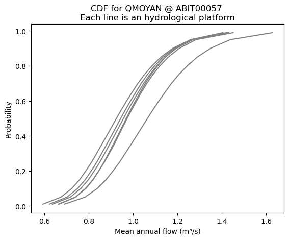
Due to their probabilistic nature, the historical reference values cannot be easily combined with the future deltas. To address this, the xhydro.cc.weighted_random_sampling and xhydro.cc.sampled_indicators functions have been designed. Together, these functions will:
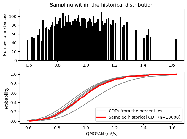
Sample ‘n’ values from the historical distribution, in accordance with the ‘percentile’ dimension.
Sample ‘n’ values from the delta distribution, using the provided weights.
Create the future distribution by applying the sampled deltas to the sampled historical distribution element-wise.
Compute the percentiles of the future distribution.
First, we will sample within the reference dataset to combine the results of the 6 hydrological platforms together.
[23]:
Help on function weighted_random_sampling in module xhydro.cc:

weighted_random_sampling(
    ds: xr.Dataset,
    *,
    weights: xr.DataArray | None = None,
    include_dims: list[str] | None = None,
    n: int = 5000,
    seed: int | None = None
) -> xr.Dataset
    Sample from a dataset using random sampling.

    Parameters
    ----------
    ds : xr.Dataset
        Dataset to sample from.
    weights : xr.DataArray, optional
        Weights to use when sampling the dataset, for dimensions other than 'percentile' or 'quantile'.
        See Notes for more information on special cases for 'percentile', 'quantile', 'time', and 'horizon' dimensions.
    include_dims : list of str, optional
        List of dimensions to include when sampling the dataset, in addition to the 'percentile' or 'quantile' dimensions and those with weights.
        These dimensions will be sampled uniformly.
    n : int
        Number of samples to generate.
    seed : int, optional
        Seed to use for the random number generator.

    Returns
    -------
    xr.Dataset
        Dataset containing the 'n' samples, stacked along a 'sample' dimension.

    Notes
    -----
    If the dataset contains a "percentile" [0, 100] or "quantile" [0, 1] dimension, the percentiles will be sampled accordingly as to
    account for the uneven spacing between percentiles and maintain the distribution's shape.

    Weights along the 'time' or 'horizon' dimensions are supported, but behave differently than other dimensions. They will not
    be stacked alongside other dimensions in the new 'sample' dimension. Rather, a separate sampling will be done for each time/horizon,
[24]:
deltas = xclim.ensembles.create_ensemble(ds_dict_deltas)

hist_dist = xh.cc.weighted_random_sampling(
    ds=ref,
    include_dims=["platform"],
    n=10000,
    seed=0,
)

hist_dist
[24]:
<xarray.Dataset> Size: 4MB
Dimensions:        (station: 2, sample: 10000)
Coordinates:
  * station        (station) <U9 72B 'ABIT00057' 'ABIT00058'
  * sample         (sample) int64 80kB 0 1 2 3 4 5 ... 9995 9996 9997 9998 9999
    lat            (station) float32 8B dask.array<chunksize=(2,), meta=np.ndarray>
    lon            (station) float32 8B dask.array<chunksize=(2,), meta=np.ndarray>
    drainage_area  (station) float32 8B dask.array<chunksize=(2,), meta=np.ndarray>
    realization    (sample) <U86 3MB dask.array<chunksize=(10000,), meta=np.ndarray>
Data variables:
    QMOYAN         (station, sample) float32 80kB dask.array<chunksize=(2, 10000), meta=np.ndarray>
Attributes: (12/29)
    title:                          Analyse des indicateurs hydrologiques aux...
    summary:                        Hydrological indicator analysis
    institution:                    DEH (Direction de l'Expertise Hydrique)
    institute_id:                   DEH
    contact:                        edouard.mailhot@environnement.gouv.qc.ca
    date_created:                   2020-10-30
    ...                             ...
    cat:frequency:                  fx
    cat:variable:                   QMOYAN
    cat:type:                       reconstruction-hydro
    cat:processing_level:           indicators
    cat:xrfreq:                     fx
cat:id: PortraitHydro_HYDROTEL_MG24HS_GovQc_GCQ_QC[25]:
# Let's show how the historical distribution was sampled and reconstructed
def _make_cdf(ds, bins):
    count, bins_count = np.histogram(ds.QMOYAN.isel(station=0), bins=bins)
    pdf = count / sum(count)
    return bins_count, np.cumsum(pdf)


# Barplot
plt.subplot(2, 1, 1)
uniquen = np.unique(hist_dist.QMOYAN.isel(station=0), return_counts=True)
plt.bar(uniquen[0], uniquen[1], width=0.01, color="k")
plt.ylabel("Number of instances")
plt.title("Sampling within the historical distribution")

# CDF
plt.subplot(2, 1, 2)
for i, platform in enumerate(ref.platform):
    plt.plot(
        ref.QMOYAN.isel(station=0).sel(platform=platform),
        ref.percentile / 100,
        "grey",
        label="CDFs from the percentiles" if i == 0 else None,
    )
bc, c = _make_cdf(hist_dist, bins=50)
plt.plot(bc[1:], c, "r", label=f"Sampled historical CDF (n={10000})", linewidth=3)
plt.ylabel("Probability")
plt.xlabel("QMOYAN (m³/s)")
plt.legend()

plt.tight_layout()
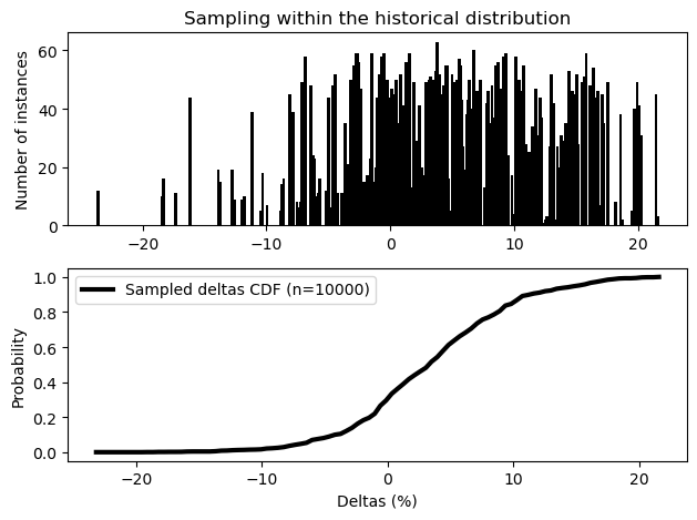
We can do the same for the deltas. Since weights already contains all dimensions that we want to sample from, we don’t need include_dims here.
[26]:
delta_dist = xh.cc.weighted_random_sampling(
    ds=deltas,
    weights=weights,
    n=10000,
    seed=0,
)

delta_dist
[26]:
<xarray.Dataset> Size: 320kB
Dimensions:        (station: 2, horizon: 3, sample: 10000)
Coordinates:
  * station        (station) <U9 72B 'ABIT00057' 'ABIT00058'
  * horizon        (horizon) <U9 108B '2021-2051' '2041-2071' '2071-2100'
  * sample         (sample) int64 80kB 0 1 2 3 4 5 ... 9995 9996 9997 9998 9999
    lat            (station) float32 8B dask.array<chunksize=(2,), meta=np.ndarray>
    lon            (station) float32 8B dask.array<chunksize=(2,), meta=np.ndarray>
    drainage_area  (station) float32 8B dask.array<chunksize=(2,), meta=np.ndarray>
Data variables:
    QMOYAN         (station, horizon, sample) float32 240kB dask.array<chunksize=(2, 3, 10000), meta=np.ndarray>
Attributes: (12/44)
    title:                          Simulation Atlas Hydroclimatique 2020
    summary:                        Derive relative des indicateurs hydrologi...
    institution:                    DEH (Direction de l'Expertise Hydrique)
    institute_id:                   DEH
    contact:                        atlas.hydroclimatique@environnement.gouv....
    date_created:                   2020-11-23
    ...                             ...
    cat:bias_adjust_project:        INFO-Crue-CM5
    cat:mip_era:                    CMIP5
    cat:activity:                   CMIP5
    cat:experiment:                 rcp45
    cat:member:                     r6i1p1
cat:bias_adjust_institution: OURANOS[27]:
# Then, let's show how the deltas were sampled, for the last horizon
plt.subplot(2, 1, 1)
uniquen = np.unique(delta_dist.QMOYAN.isel(station=0, horizon=-1), return_counts=True)
plt.bar(uniquen[0], uniquen[1], width=0.25, color="k")
plt.ylabel("Number of instances")
plt.title("Sampling within the historical distribution")

plt.subplot(2, 1, 2)
bc, c = _make_cdf(delta_dist, bins=100)
plt.plot(bc[1:], c, "k", label=f"Sampled deltas CDF (n={10000})", linewidth=3)
plt.ylabel("Probability")
plt.xlabel("Deltas (%)")
plt.legend()

plt.tight_layout()
Once the two distributions have been acquired, xhydro.cc.sampled_indicators can be used to combine them element-wise and reconstruct a future distribution. The resulting distribution will possess the unique dimensions from both datasets. Here, this means that we get a reconstructed distribution for each future horizon.
[28]:
help(xh.cc.sampled_indicators)
Help on function sampled_indicators in module xhydro.cc:

sampled_indicators(
    ds_dist: xr.Dataset,
    deltas_dist: xr.Dataset,
    *,
    delta_kind: str | dict | None = None,
    percentiles: xr.DataArray | xr.Dataset | list[int] | np.ndarray | None = None
) -> xr.Dataset | tuple[xr.Dataset, xr.Dataset]
    Reconstruct indicators using a perturbation approach and random sampling.

    Parameters
    ----------
    ds_dist : xr.Dataset
        Dataset containing the sampled reference distribution, stacked along a 'sample' dimension.
        Typically generated using 'xhydro.cc.weighted_random_sampling'.
    deltas_dist : xr.Dataset
        Dataset containing the sampled deltas, stacked along a 'sample' dimension.
        Typically generated using 'xhydro.cc.weighted_random_sampling'.
    delta_kind : str or dict, optional
        Type of delta provided. Recognized values are: ['absolute', 'abs.', '+'], ['percentage', 'pct.', '%'].
        If a dict is provided, it should map the variable names to their respective delta type.
        If None, the variables should have a 'delta_kind' attribute.
    percentiles : xr.DataArray or xr.Dataset or list or np.ndarray, optional
        Percentiles to compute in the future distribution.
        This will change the output of the function to a tuple containing the future distribution and the future percentiles.
        If given a Dataset, it should contain a 'percentile' or 'quantile' dimension.
        If given a list or np.ndarray, it should contain percentiles [0, 100].

    Returns
    -------
    fut_dist : xr.Dataset
        The future distribution, stacked along the 'sample' dimension.
    fut_pct : xr.Dataset
        Dataset containing the future percentiles.

    Notes
    -----
    The future percentiles are computed as follows:
    1. Sample 'n' values from the reference distribution.
    2. Sample 'n' values from the delta distribution.
    3. Create the future distribution by applying the sampled deltas to the sampled historical distribution, element-wise.
    4. Compute the percentiles of the future distribution (optional).
[29]:
fut_dist, fut_pct = xh.cc.sampled_indicators(
    ds_dist=hist_dist,
    deltas_dist=delta_dist,
    delta_kind="percentage",
    percentiles=ref.percentile,
)

fut_dist
WARNING:xscen.utils:Unable to generate a new id for the dataset. Got single positional indexer is out-of-bounds.
[29]:
<xarray.Dataset> Size: 4MB
Dimensions:        (station: 2, sample: 10000, horizon: 3)
Coordinates:
  * station        (station) <U9 72B 'ABIT00057' 'ABIT00058'
  * sample         (sample) int64 80kB 0 1 2 3 4 5 ... 9995 9996 9997 9998 9999
  * horizon        (horizon) <U9 108B '2021-2051' '2041-2071' '2071-2100'
    lat            (station) float32 8B dask.array<chunksize=(2,), meta=np.ndarray>
    lon            (station) float32 8B dask.array<chunksize=(2,), meta=np.ndarray>
    drainage_area  (station) float32 8B dask.array<chunksize=(2,), meta=np.ndarray>
    realization    (sample) <U86 3MB dask.array<chunksize=(10000,), meta=np.ndarray>
Data variables:
QMOYAN (station, sample, horizon) float32 240kB dask.array<chunksize=(2, 10000, 3), meta=np.ndarray>Since we used the percentiles argument, it also computed a series of percentiles.
[30]:
fut_pct
[30]:
<xarray.Dataset> Size: 1kB
Dimensions:        (station: 2, horizon: 3, percentile: 21)
Coordinates:
  * station        (station) <U9 72B 'ABIT00057' 'ABIT00058'
  * horizon        (horizon) <U9 108B '2021-2051' '2041-2071' '2071-2100'
  * percentile     (percentile) float32 84B 1.0 5.0 10.0 15.0 ... 90.0 95.0 99.0
    lat            (station) float32 8B dask.array<chunksize=(2,), meta=np.ndarray>
    lon            (station) float32 8B dask.array<chunksize=(2,), meta=np.ndarray>
    drainage_area  (station) float32 8B dask.array<chunksize=(2,), meta=np.ndarray>
Data variables:
QMOYAN (percentile, station, horizon) float64 1kB dask.array<chunksize=(21, 2, 3), meta=np.ndarray>[31]:
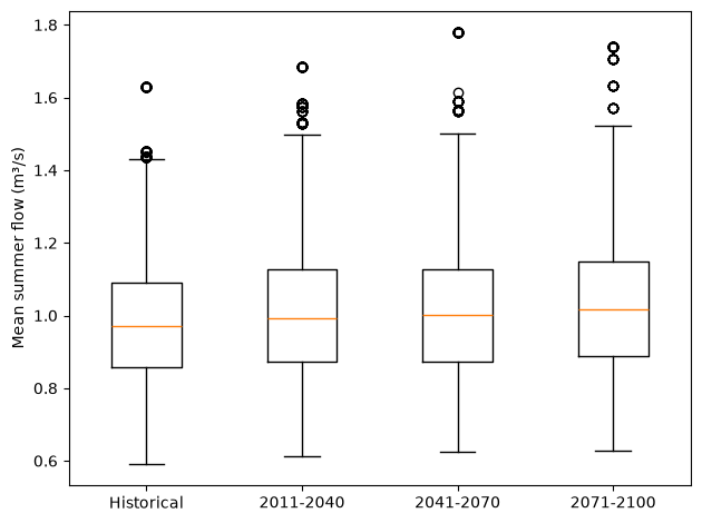
# The distributions themselves can be used to create boxplots and compare the historical distribution to the future ones.
plt.boxplot(
    [
        hist_dist.QMOYAN.isel(station=0),
        fut_dist.QMOYAN.isel(station=0, horizon=0),
        fut_dist.QMOYAN.isel(station=0, horizon=1),
        fut_dist.QMOYAN.isel(station=0, horizon=2),
    ],
    tick_labels=["Historical", "2011-2040", "2041-2070", "2071-2100"],
)

plt.ylabel("Mean summer flow (m³/s)")
plt.tight_layout()
The same statistics as before can also be computed by using the 10,000 samples within delta_dist.
[32]:
# The same statistics as before can also be computed by using delta_dist
delta_dist = delta_dist.rename({"sample": "realization"})  # xclim compatibility
ens_stats = xh.cc.ensemble_stats(delta_dist, statistics)

out_prob = xr.Dataset()
out_prob["QMOYAN_median"] = ens_stats["QMOYAN"].sel(percentiles=50)
out_prob["QMOYAN_iqr"] = ens_stats["QMOYAN"].sel(percentiles=75) - ens_stats[
    "QMOYAN"
].sel(percentiles=25)
out_prob["QMOYAN_robustness_categories"] = robustness_categories(
    changed_or_fractions=ens_stats["QMOYAN_changed"],
    agree=ens_stats["QMOYAN_positive"],
    categories=categories,
    thresholds=thresholds,
    ops=ops,
)

out_prob
[32]:
<xarray.Dataset> Size: 308B
Dimensions:                       (station: 2, horizon: 3)
Coordinates:
  * station                       (station) <U9 72B 'ABIT00057' 'ABIT00058'
  * horizon                       (horizon) <U9 108B '2021-2051' ... '2071-2100'
    lat                           (station) float32 8B dask.array<chunksize=(2,), meta=np.ndarray>
    lon                           (station) float32 8B dask.array<chunksize=(2,), meta=np.ndarray>
    drainage_area                 (station) float32 8B dask.array<chunksize=(2,), meta=np.ndarray>
    percentiles                   int64 8B 50
Data variables:
    QMOYAN_median                 (station, horizon) float32 24B dask.array<chunksize=(2, 3), meta=np.ndarray>
    QMOYAN_iqr                    (station, horizon) float32 24B dask.array<chunksize=(2, 3), meta=np.ndarray>
    QMOYAN_robustness_categories  (station, horizon) int64 48B dask.array<chunksize=(2, 3), meta=np.ndarray>