5. Optimal interpolation¶

Optimal interpolation is a method used to combine spatially distributed data (the “background field”) with point-based observations. This technique adjusts the entire field by incorporating deviations between the observed data and the field at the observation points, resulting in a statistically optimal adjustment of the background field. For example, it can be used to blend reanalysis precipitation data (such as ERA5) with actual observational records, ensuring that the reanalysis precipitation is corrected over the entire domain.

This page demonstrates how to use xHydro to perform optimal interpolation for hydrological modeling by integrating field-like simulations with point observations. In this case, the background field consists of outputs from a distributed hydrological model, while the point observations correspond to real hydrometric station measurements. The goal is to correct the background field (i.e., the hydrological model outputs) using optimal interpolation techniques, following the approach outlined in Lachance-Cloutier et al. (2017).

Lachance-Cloutier, S., Turcotte, R. and Cyr, J.F., 2017. Combining streamflow observations and hydrologic simulations for the retrospective estimation of daily streamflow for ungauged rivers in southern Quebec (Canada). Journal of hydrology, 550, pp.294-306.

Optimal interpolation relies on a set of hyperparameters. Some of these are more complex than others, so let’s break down the main steps.

The first step is to compute the differences (or “departures”) between the observed and simulated flow at the stations where both values are available. These differences must be scaled by the catchment area to ensure that errors are relative and can be properly interpolated. Also, we take the logarithm of these scaled values to prevent negative streamflow during extrapolation. We will reverse this transformation later in the process.

Next, we need some additional information, which may or may not be available for our observation and simulation sites. These include estimates of:

The variance of the observations at the gauged sites.
The variance of the simulated flows at the observation sites.
The variance of the simulated flows at the estimation sites, including those that also correspond to an observation site.

These can be estimated in real-world applications using long time series of log-transformed and scaled flows, or from measurement errors associated with the instrumentation at gauged sites. These parameters can also be fine-tuned based on past experience or through trial-and-error.

The final component we need is the error covariance function (ECF). In simple terms, optimal interpolation takes into account the distance between an observation (or multiple observations) and the site where we need to estimate a new flow value. Intuitively, a simulation station close to an observation station should have a high correlation with it, while a station farther away will have a lower correlation. Therefore, we need a covariance function that estimates:

The degree of covariability between an observed and simulated point.
The distance between these points.

The ECF function is key to this, and several models of it exist in the literature. In many cases, a model form will be chosen a priori, and its parameters will be adjusted to best represent the covariance between points.

In this test example, we don’t have enough points or time steps to develop a meaningful model (or parameterization) from the data. As a result, we will impose a model. xHydro includes four built-in models, where par[0] and par[1] are the model parameters to be calibrated (under normal circumstances), and h represents the distance between points:

Model 1:

\[\begin{flalign*} &\text{par}[0] \cdot \left( 1 + \frac{h}{\text{par}[1]} \right) \cdot \exp\left(- \frac{h}{\text{par}[1]} \right) && \text{— From Lachance-Cloutier et al. 2017.} \end{flalign*}\]
Model 2:

\[\begin{flalign*} &\text{par}[0] \cdot \exp\left( -0.5 \cdot \left( \frac{h}{\text{par}[1]} \right)^2 \right) && \end{flalign*}\]
Model 3:

\[\begin{flalign*} &\text{par}[0] \cdot \exp\left( -\frac{h}{\text{par}[1]} \right) && \end{flalign*}\]
Model 4:

\[\begin{flalign*} &\text{par}[0] \cdot \exp\left( -\frac{h^{\text{par}[1]}}{\text{par}[0]} \right) && \end{flalign*}\]

[1]:

import datetime as dt
from functools import partial
from pathlib import Path

import matplotlib.pyplot as plt
import numpy as np
import pandas as pd
import pooch
import xarray as xr
from scipy.stats import norm

import xhydro as xh
import xhydro.optimal_interpolation
from xhydro.testing.helpers import deveraux

ERROR 1: PROJ: proj_create_from_database: Open of /home/docs/checkouts/readthedocs.org/user_builds/xhydro/conda/stable/share/proj failed
/home/docs/checkouts/readthedocs.org/user_builds/xhydro/conda/stable/lib/python3.14/site-packages/xhydro/__init__.py:21: UserWarning: The `exactextract` library is not present in the environment and will not be used.

5.1. Example with HYDROTEL data¶

Optimal interpolation relies on both observed and simulated datasets and requires the following information:

Observed data for the gauged locations
Simulated data for all locations
Catchment areas (for error scaling)
Catchment latitude and longitude (to develop the spatial error model)

This example will use a subset of data generated using the HYDROTEL hydrological model.

[2]:

# Get data
test_data_path = deveraux().fetch(
    "optimal_interpolation/OI_data_corrected.zip",
    pooch.Unzip(),
)
directory_to_extract_to = Path(test_data_path[0]).parent

# Read-in all the files and set to paths that we can access later.
qobs = xr.open_dataset(directory_to_extract_to / "A20_HYDOBS_TEST_corrected.nc").rename(
    {"streamflow": "q"}
)
qsim = xr.open_dataset(directory_to_extract_to / "A20_HYDREP_TEST_corrected.nc").rename(
    {"streamflow": "q"}
)
station_correspondence = xr.open_dataset(
    directory_to_extract_to / "station_correspondence.nc"
)
df_validation = pd.read_csv(
    directory_to_extract_to / "stations_retenues_validation_croisee.csv",
    dtype=str,
)
observation_stations = list(df_validation["No_station"])

There are three datasets, as well as a list:

qobs: The dataset containing point observations and station metadata.
qsim: The dataset containing the background field simulations (e.g. the raw HYDROTEL results), including simulated station metadata.
station_correspondence: A dataset that simply links station identifiers between the observed and simulated stations. This is necessary because observed stations use “real-world” identifiers, while distributed simulations often employ coded or sequentially numbered identifiers.
observation_stations: A list of the stations from the observation set that we want to use to build the optimal interpolation.

[3]:

qobs

[4]:

qsim

[5]:

station_correspondence

[5]:

<xarray.Dataset> Size: 18kB
Dimensions:     (station: 296)
Dimensions without coordinates: station
Data variables:
    reach_id    (station) <U9 11kB ...
    station_id  (station) <U6 7kB ...

[6]:

print(
    f"There are a total of {len(observation_stations)} selected observation stations."
)
print(observation_stations)

There are a total of 96 selected observation stations.
['011508', '011509', '020602', '020802', '021601', '021915', '021916', '022003', '022301', '022601', '022704', '023303', '023401', '023402', '023702', '024003', '024007', '024010', '024014', '024015', '030101', '030103', '030215', '030234', '030282', '030335', '030345', '030424', '030425', '030905', '030907', '030919', '030921', '040129', '040204', '040841', '040830', '040840', '041902', '041903', '042103', '043012', '050144', '050135', '050304', '050408', '050409', '050702', '050801', '050812', '050915', '050916', '051001', '051005', '051006', '051301', '051502', '052228', '052231', '052601', '052606', '052805', '060101', '060102', '060202', '060601', '060704', '060901', '061020', '061022', '061024', '061028', '061307', '061502', '061801', '061901', '061905', '061909', '062102', '062114', '062701', '062803', '070401', '072301', '073502', '073503', '073801', '074701', '074902', '075702', '075705', '076201', '076601', '080101', '080106', '080707']

WARNING

The optimal interpolation module in xHydro is still a work-in-progress and is highly hard-coded, particularly regarding inputs. Expect significant changes as the code is refactored and improved.

The datasets need to follow specific formatting requirements.

For the observed dataset (qobs in this example), the following conditions must be met:

The dimensions should be station and time.
The streamflow data must be stored in a variable called streamflow.
The catchment drainage area must be represented in a variable named drainage_area.
The latitude and longitude of the catchment centroids must be stored as centroid_lat and centroid_lon (these are not the hydrometric station coordinates).
A variable called station_id must exist, containing a unique identifier for each station. This will be used to match the observation stations with their corresponding simulated stations.

For the simulation dataset (qsim in this example), the following requirements apply:

The dimensions should be station and time.
The streamflow data should be in a variable named streamflow.
The drainage area for each catchment, as simulated by the model, should be stored in a variable called drainage_area.
The centroids of the catchments must be represented by the coordinates lat and lon.
A variable called station_id must exist, containing a unique identifier for each simulated station, used to map it to the observed stations.

The correspondence table (station_correspondence in this example) must include:

station_id for the observed stations.
reach_id for the simulated stations.

Optimal interpolation in xHydro is primarily accessed through the xhydro.optimal_interpolation.optimal_interpolation_fun.execute_interpolation function. When performing leave-one-out cross-validation across multiple catchments, the entire interpolation process is repeated for each catchment. In each iteration, one observation station is left out and held independent for validation. This process can be time-consuming but can be parallelized by adjusting the relevant flag and setting the number of CPU cores based on your machine’s capacity. By default, the code will use only 1 core, but if you choose to increase it, the maximum number of cores used will be limited to ([number-of-available-cores / 2] - 1) to avoid overloading your computer.

[7]:

help(xhydro.optimal_interpolation.execute)

Help on function execute_interpolation in module xhydro.optimal_interpolation.optimal_interpolation_fun:

execute_interpolation(
qobs: xr.Dataset,
qsim: xr.Dataset,
station_correspondence: xr.Dataset,
observation_stations: list,
ratio_var_bg: float = 0.15,
percentiles: list[float] | None = None,
variogram_bins: int = 10,
parallelize: bool = False,
max_cores: int = 1,
leave_one_out_cv: bool = False,
form: int = 3,
hmax_divider: float = 2.0,
p1_bnds: list | None = None,
hmax_mult_range_bnds: list | None = None
) -> xr.Dataset
Run the interpolation algorithm for leave-one-out cross-validation or operational use.

Parameters
----------
qobs : xr.Dataset
Streamflow and catchment properties dataset for observed data.
qsim : xr.Dataset
Streamflow and catchment properties dataset for simulated data.
station_correspondence : xr.Dataset
Correspondence between the tag in the simulated files and the observed station number for the obs dataset.
observation_stations : list
Observed hydrometric dataset stations to be used in the ECF function building and optimal interpolation
application step.
ratio_var_bg : float
Ratio for background variance (default is 0.15).
percentiles : list(float), optional
List of percentiles to analyze (default is [25.0, 50.0, 75.0, 100.0]).
variogram_bins : int, optional
Number of bins to split the data to fit the semi-variogram for the ECF. Defaults to 10.
parallelize : bool
Execute the profiler in parallel or in series (default is False).
max_cores : int
Maximum number of cores to use for parallel processing.
leave_one_out_cv : bool
Flag to determine if the code should be run in leave-one-out cross-validation (True) or should be applied
operationally (False).
form : int
The form of the ECF equation to use (1, 2, 3 or 4. See documentation).
hmax_divider : float
Maximum distance for binning is set as hmax_divider times the maximum distance in the input data. Defaults to 2.
p1_bnds : list, optional
The lower and upper bounds of the parameters for the first parameter of the ECF equation for variogram fitting.
Defaults to [0.95, 1].
hmax_mult_range_bnds : list, optional
The lower and upper bounds of the parameters for the second parameter of the ECF equation for variogram fitting.
It is multiplied by "hmax", which is calculated to be the threshold limit for the variogram sill.
Defaults to [0.05, 3].

Returns
-------
xr.Dataset
An xarray dataset containing the flow quantiles and all the associated metadata.

[8]:

ds = xh.optimal_interpolation.execute(
    qobs=qobs.sel(time=slice("2018-11-01", "2019-01-01")),
    qsim=qsim.sel(time=slice("2018-11-01", "2019-01-01")),
    station_correspondence=station_correspondence,
    observation_stations=observation_stations,
    form=1,
    ratio_var_bg=0.15,
    percentiles=[25, 50, 75],
    parallelize=False,
    max_cores=1,
    leave_one_out_cv=False,
)

ds

The returned dataset contains a streamflow variable called q with the dimensions [percentile, station_id, time], providing estimates for any requested percentile to assess uncertainty. Let’s now explore how the optimal interpolation has changed the streamflow at one catchment.

[9]:

# Get a pair of station ID at one of the stations used for optimal interpolation
pair = station_correspondence.where(
    station_correspondence.station_id == observation_stations[0], drop=True
)
obs_id = pair["station_id"].data
sim_id = pair["reach_id"].data

# Get the streamflow data
observed_flow_select = (
    qobs["q"]
    .where(qobs.station_id == obs_id, drop=True)
    .sel(time=slice("2018-11-01", "2019-01-01"))
    .squeeze()
)
raw_simulated_flow_select = (
    qsim["q"]
    .where(qsim.station_id == sim_id, drop=True)
    .sel(time=slice("2018-11-01", "2019-01-01"))
    .squeeze()
)
interpolated_flow_select = ds["q"].sel(
    station_id=sim_id[0], percentile=50.0, time=slice("2018-11-01", "2019-01-01")
)

[10]:

plt.plot(observed_flow_select, label="Observed flow")
plt.plot(raw_simulated_flow_select, label="Raw simulation")
plt.plot(interpolated_flow_select, label="Interpolated simulation")
plt.xlabel("Simulation day")
plt.ylabel("Streamflow (m³/s)")
plt.legend()
plt.show()

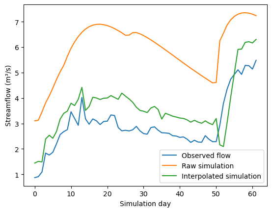
../_images/notebooks_optimal_interpolation_16_0.png

We can observe that optimal interpolation generally helped bring the model simulation closer to the observed data.