Use Case Example
This example illustrates a use case that covers the essential steps involved in building a hydrological model and conducting a climate change analysis:
Identification of the watershed and its key characteristics
Beaurivage watershed in Southern Quebec, at the location of the 023401 streamflow gauge.
Collection of observed data
ERA5-Land and streamflow gauge data.
Preparation and calibration of the hydrological model
GR4JCN emulated by the Raven hydrological framework.
Calculation of hydrological indicators
Mean summer flow
Mean monthly flow
20- and 100-year maximum flow
2-year minimum 7-day average summer flow
Assessment of the impact of climate change
Bias-adjusted CMIP6 simulations from the ESPO-G6-R2 dataset
Identification of a watershed and its characteristics
INFO
For more information on this section and available options, consult the GIS notebook.
This first step is highly dependent on the hydrological model. Since we will use GR4JCN in our example, we need to obtain the drainage area, centroid coordinates, and elevation. We’ll also need the watershed delineation to extract the meteorological data. All of these information can be acquired through the xhydro.gis.watershed_to_raven_hru function, which calls upon various functions of that module.
[1]:
import warnings
warnings.filterwarnings("ignore", category=UserWarning)
warnings.filterwarnings("ignore", category=FutureWarning)
[2]:
from IPython.display import clear_output

import xhydro.gis as xhgis

clear_output(wait=False)
[3]:
# Watershed delineation
coords = (-71.28878, 46.65692)
gdf = xhgis.watershed_to_raven_hru(coords)
gdf
[3]:
| HRU_ID | area | latitude | longitude | elevation | SubId | DowSubId | geometry | |
|---|---|---|---|---|---|---|---|---|
| 0 | 7120365812 | 585.585577 | 46.452161 | -71.260464 | 222.55365 | 1 | -1 | POLYGON ((-71.09758 46.40035, -71.09409 46.403... |
Since xhgis.watershed_delineation extracts the nearest HydroBASINS polygon, the watershed might not exactly correspond to the requested coordinates. The 023401 streamflow gauge as an associated drainage area of 708 km², which differs from our results. Streamflow will have to be adjusted using an area scaling factor.
[4]:
gauge_area = 708
scaling_factor = gdf.iloc[0]["area"] / gauge_area
scaling_factor
[4]:
np.float64(0.8270982719703007)
Collection of observed data
[5]:
import geopandas as gpd
import matplotlib.pyplot as plt
import xarray as xr

# For easy access to the specific streamflow data used here
import xdatasets
import xscen
Meteorological data
INFO
Multiple libraries could be used to perform these steps. For simplicity, this example will use the subset and aggregate modules of the xscen library.
This example will use daily ERA5-Land data hosted on the PAVICS platform.
[6]:
# Extraction of ERA5-Land data
meteo_ref = xr.open_dataset(
    "https://pavics.ouranos.ca/twitcher/ows/proxy/thredds/dodsC/datasets/reanalyses/day_ERA5-Land_NAM.ncml",
    engine="netcdf4",
    chunks={"time": 365, "lon": 50, "lat": 50},
)[["pr", "tasmin", "tasmax"]]
meteo_ref
[6]:
<xarray.Dataset> Size: 454GB
Dimensions:  (time: 27790, lat: 801, lon: 1700)
Coordinates:
  * time     (time) datetime64[ns] 222kB 1950-01-01 1950-01-02 ... 2026-01-31
  * lat      (lat) float32 3kB 10.0 10.1 10.2 10.3 10.4 ... 89.7 89.8 89.9 90.0
  * lon      (lon) float32 7kB -179.9 -179.8 -179.7 -179.6 ... -10.2 -10.1 -10.0
Data variables:
    pr       (time, lat, lon) float32 151GB dask.array<chunksize=(365, 50, 50), meta=np.ndarray>
    tasmin   (time, lat, lon) float32 151GB dask.array<chunksize=(365, 50, 50), meta=np.ndarray>
    tasmax   (time, lat, lon) float32 151GB dask.array<chunksize=(365, 50, 50), meta=np.ndarray>
Attributes: (12/30)
    Conventions:               CF-1.9
    cell_methods:              time: mean (interval: 1 day)
    doi:                       https://doi.org/10.24381/cds.e2161bac
    domain:                    NAM
    frequency:                 day
    history:                   [2022-12-25 09:07:39.901698] Converted variabl...
    ...                        ...
    institute_id:              ECMWF
    dataset_id:                ERA5-Land
    abstract:                  ERA5-Land provides hourly high resolution info...
    dataset_description:       https://www.ecmwf.int/en/era5-land
    attribution:               Contains modified Copernicus Climate Change Se...
citation: Muñoz Sabater, J., (2021): ERA5-Land hourly da...That dataset covers the entire globe and has more than 70 years of data. The first step will thus be to subset the dataset both spatially and temporally. For the spatial subset, the GeoDataFrame obtained earlier can be used.
[7]:
meteo_ref = meteo_ref.sel(time=slice("1991", "2020"))  # Temporal subsetting
meteo_ref = xscen.spatial.subset(
    meteo_ref, method="shape", tile_buffer=2, shape=gdf
)  # Spatial subsetting, with a buffer of 2 grid cells
meteo_ref
[7]:
<xarray.Dataset> Size: 9MB
Dimensions:  (time: 10958, lat: 8, lon: 8)
Coordinates:
  * time     (time) datetime64[ns] 88kB 1991-01-01 1991-01-02 ... 2020-12-31
  * lat      (lat) float32 32B 46.1 46.2 46.3 46.4 46.5 46.6 46.7 46.8
  * lon      (lon) float32 32B -71.6 -71.5 -71.4 -71.3 -71.2 -71.1 -71.0 -70.9
Data variables:
    pr       (time, lat, lon) float32 3MB dask.array<chunksize=(355, 8, 8), meta=np.ndarray>
    tasmin   (time, lat, lon) float32 3MB dask.array<chunksize=(355, 8, 8), meta=np.ndarray>
    tasmax   (time, lat, lon) float32 3MB dask.array<chunksize=(355, 8, 8), meta=np.ndarray>
Attributes: (12/30)
    Conventions:               CF-1.9
    cell_methods:              time: mean (interval: 1 day)
    doi:                       https://doi.org/10.24381/cds.e2161bac
    domain:                    NAM
    frequency:                 day
    history:                   [2026-03-31 14:35:41] shape spatial subsetting...
    ...                        ...
    institute_id:              ECMWF
    dataset_id:                ERA5-Land
    abstract:                  ERA5-Land provides hourly high resolution info...
    dataset_description:       https://www.ecmwf.int/en/era5-land
    attribution:               Contains modified Copernicus Climate Change Se...
citation: Muñoz Sabater, J., (2021): ERA5-Land hourly da...[8]:
ax = plt.subplot(1, 1, 1)
meteo_ref.tasmin.isel(time=0).plot(ax=ax)
gdf.plot(ax=ax)
[8]:
<Axes: title={'center': 'time = 1991-01-01'}, xlabel='longitude [degrees_east]', ylabel='latitude [degrees_north]'>
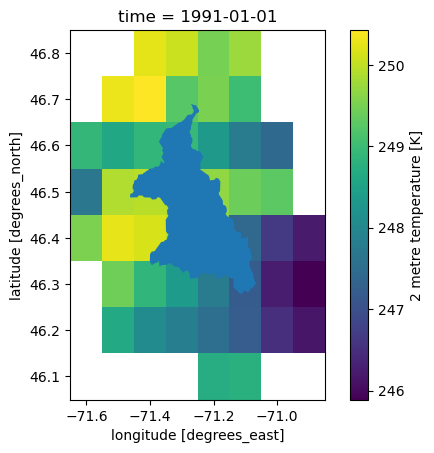
Raven expects temperatures in Celsius and precipitation in millimetres, but they currently are in CF-compliant Kelvin and kg m-2 s-1, respectively. The xhydro.modelling.format_input function can be used to prepare data for Raven modelling. It handles unit conversion, variable renaming, and coordinate formatting to ensure compatibility with RavenPy. In the case of gridded meteorological data—as in this example—xHydro calls functions available in RavenPy to assign weights to each
grid cell based on the portion that overlaps with the watershed. Alternatively, the data could be aggregated manually before being passed to the model.
For simplification matters, the grid’s elevation will be set at a flat 450 m. Computing grid cell elevation in ERA5-Land is not always trivial and is not within the scope of this example.
[9]:
from pathlib import Path
import tempfile
notebook_folder = Path(tempfile.TemporaryDirectory().name)

import xhydro as xh

# Add altitude data
meteo_ref = meteo_ref.assign_coords(
    {"elevation": xr.ones_like(meteo_ref.pr.isel(time=0).drop_vars("time")) * 450}
)
meteo_ref["elevation"].attrs = {"units": "m"}

meteo_ref, config_meteo_ref = xh.modelling.format_input(
    meteo_ref, model="GR4JCN", save_as=notebook_folder / "_data" / "meteo.nc"
)
meteo_ref
[9]:
<xarray.Dataset> Size: 9MB
Dimensions:    (time: 10958, latitude: 8, longitude: 8)
Coordinates:
  * time       (time) datetime64[ns] 88kB 1991-01-01 1991-01-02 ... 2020-12-31
  * latitude   (latitude) float32 32B 46.1 46.2 46.3 46.4 46.5 46.6 46.7 46.8
  * longitude  (longitude) float32 32B -71.6 -71.5 -71.4 ... -71.1 -71.0 -70.9
    elevation  (latitude, longitude) float32 256B dask.array<chunksize=(8, 8), meta=np.ndarray>
Data variables:
    pr         (time, latitude, longitude) float32 3MB dask.array<chunksize=(355, 8, 8), meta=np.ndarray>
    tasmin     (time, latitude, longitude) float32 3MB dask.array<chunksize=(355, 8, 8), meta=np.ndarray>
    tasmax     (time, latitude, longitude) float32 3MB dask.array<chunksize=(355, 8, 8), meta=np.ndarray>
Attributes: (12/30)
    Conventions:               CF-1.9
    cell_methods:              time: mean (interval: 1 day)
    doi:                       https://doi.org/10.24381/cds.e2161bac
    domain:                    NAM
    frequency:                 day
    history:                   [2026-03-31 14:35:41] shape spatial subsetting...
    ...                        ...
    institute_id:              ECMWF
    dataset_id:                ERA5-Land
    abstract:                  ERA5-Land provides hourly high resolution info...
    dataset_description:       https://www.ecmwf.int/en/era5-land
    attribution:               Contains modified Copernicus Climate Change Se...
citation: Muñoz Sabater, J., (2021): ERA5-Land hourly da...That function also returns information that will be used later to instanciate the hydrological model:
[10]:
config_meteo_ref
[10]:
{'data_type': ['TEMP_MAX', 'TEMP_MIN', 'PRECIP'],
 'alt_names_meteo': {'TEMP_MAX': 'tasmax',
  'TEMP_MIN': 'tasmin',
  'PRECIP': 'pr'},
 'meteo_file': '/tmp/tmpbnxtefbc/_data/meteo.nc'}
Hydrometric data
Gauge streamflow data from the Quebec government can be accessed through the xdatasets library.
[11]:
qobs = (
    xdatasets.Query(
        **{
            "datasets": {
                "deh": {
                    "id": ["023401"],
                    "variables": ["streamflow"],
                }
            },
            "time": {"start": "1991-01-01", "end": "2020-12-31"},
        }
    )
    .data.squeeze()
    .load()
).sel(spatial_agg="watershed")
[12]:
# Once again, some housekeeping is required on the metadata to make sure that xHydro understands the dataset.
qobs = qobs.rename({"streamflow": "q"})
qobs["id"].attrs["cf_role"] = "timeseries_id"
qobs = qobs.rename({"id": "station_id"})
qobs["q"].attrs = {
    "long_name": "Streamflow",
    "units": "m3 s-1",
    "standard_name": "water_volume_transport_in_river_channel",
    "cell_methods": "time: mean",
}
for c in qobs.coords:
    if len(qobs[c].dims) == 0 and "time" not in c:
        qobs[c] = qobs[c].expand_dims("station_id")

qobs
[12]:
<xarray.Dataset> Size: 132kB
Dimensions:        (time: 10958, station_id: 1)
Coordinates: (12/15)
  * time           (time) datetime64[ns] 88kB 1991-01-01 ... 2020-12-31
  * station_id     (station_id) <U6 24B '023401'
    drainage_area  (station_id) float32 4B 708.0
    end_date       (station_id) datetime64[ns] 8B 2020-12-31
    latitude       (station_id) float32 4B 46.66
    longitude      (station_id) float32 4B -71.29
    ...             ...
    source         (station_id) <U102 408B 'Ministère de l’Environnement, de ...
    spatial_agg    (station_id) <U9 36B 'watershed'
    start_date     (station_id) datetime64[ns] 8B 1991-01-01
    variable       (station_id) <U10 40B 'streamflow'
    time_agg       <U4 16B 'mean'
    timestep       <U1 4B 'D'
Data variables:
q (time) float32 44kB 46.0 33.9 26.2 21.0 ... 19.98 15.76 12.93[13]:
plt.figure(figsize=[10, 5])
qobs.q.plot()
[13]:
[<matplotlib.lines.Line2D at 0x7f5f93952ba0>]
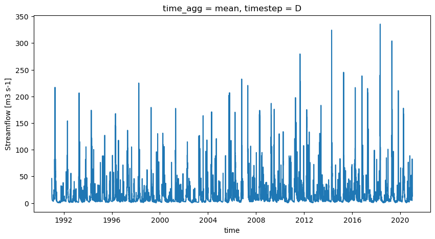
As specified earlier, streamflow observations need to be modified to account for the differences in watershed sizes between the gauge and the polygon.
[14]:
with xr.set_options(keep_attrs=True):
    qobs["q"] = qobs["q"] * scaling_factor
[15]:
# Save (necessary for model calibration)
qobs.to_netcdf(notebook_folder / "_data" / "qobs.nc")
Preparation and calibration of the hydrological model (xhydro.modelling)
INFO
For more information on this section and available options, consult the Hydrological modelling notebook.
[16]:
import xhydro as xh
from xhydro.modelling.calibration import perform_calibration
from xhydro.modelling.obj_funcs import get_objective_function
The perform_calibration function requires a model_config argument that allows it to build the corresponding hydrological model. All the required information has been acquired in previous sections, so it is only a matter of filling in the entries of the RavenPy/GR4JCN model.
For simplification matters, as snow water equivalent is not currently available on PAVICS’ database, “AVG_ANNUAL_SNOW” was roughly estimated using Brown & Brasnett (2010).
[17]:
# Model configuration
model_config = {
    "model_name": "GR4JCN",
    "workdir": notebook_folder / "model",
    "overwrite": True,
    "parameters": [0.529, -3.396, 407.29, 1.072, 16.9, 0.947],
    "hru": gdf,
    "start_date": "1991-01-01",
    "end_date": "2020-12-31",
    "rain_snow_fraction": "RAINSNOW_DINGMAN",
    "evaporation": "PET_HARGREAVES_1985",
    "global_parameter": {"AVG_ANNUAL_SNOW": 100.00},
    **config_meteo_ref,  # Reuse information gathered earlier
}

# Parameter bounds for GR4JCN
bounds_low = [0.01, -15.0, 10.0, 0.0, 1.0, 0.0]
bounds_high = [2.5, 10.0, 700.0, 7.0, 30.0, 1.0]
[18]:
# Calibration / validation period
mask_calib = xr.where(qobs.time.dt.year <= 2010, 1, 0).values
mask_valid = xr.where(qobs.time.dt.year > 2010, 1, 0).values

# Model calibration
best_parameters, best_simulation, best_objfun = perform_calibration(
    model_config,
    "kge",
    qobs=notebook_folder / "_data" / "qobs.nc",
    bounds_low=bounds_low,
    bounds_high=bounds_high,
    evaluations=8,
    algorithm="DDS",
    mask=mask_calib,
    sampler_kwargs=dict(trials=1),
)
Initializing the  Dynamically Dimensioned Search (DDS) algorithm  with  8  repetitions
The objective function will be maximized
Starting the DDS algorithm with 8 repetitions...
Finding best starting point for trial 1 using 5 random samples.
1 of 8, maximal objective function=0.129327, time remaining: 00:00:10
Initialize database...
['csv', 'hdf5', 'ram', 'sql', 'custom', 'noData']
2 of 8, maximal objective function=0.129327, time remaining: 00:00:11
3 of 8, maximal objective function=0.293959, time remaining: 00:00:09
4 of 8, maximal objective function=0.293959, time remaining: 00:00:08
5 of 8, maximal objective function=0.293959, time remaining: 00:00:05
6 of 8, maximal objective function=0.293959, time remaining: 00:00:03
7 of 8, maximal objective function=0.390197, time remaining: 00:00:00
8 of 8, maximal objective function=0.393656, time remaining: 23:59:57
Best solution found has obj function value of 0.3936562927318237 at 5


*** Final SPOTPY summary ***
Total Duration: 24.88 seconds
Total Repetitions: 8
Maximal objective value: 0.393656
Corresponding parameter setting:
param0: 1.13242
param1: -2.46413
param2: 43.5229
param3: 1.33209
param4: 24.153
param5: 0.0766439
******************************

Best parameter set:
param0=1.132418270728551, param1=-2.464133107201744, param2=43.522924628974806, param3=1.3320909887768697, param4=24.153016559360484, param5=0.07664389863678882
Run number 7 has the highest objectivefunction with: 0.3937
To reduce computation times for this example, only 10 steps were used for the calibration function, which is well below the recommended number. The parameters below were obtained by running the code above with 150 evaluations.
[19]:
# Replace the results with parameters obtained using 150 evaluations
best_parameters = [
    0.3580270511815579,
    -2.187141388684563,
    24.012067980309702,
    0.000781,
    1.9330212374187332,
    0.5491789347783598,
]
model_config["parameters"] = best_parameters

best_simulation = xh.modelling.hydrological_model(model_config).run()
The real KGE should be computed from a validation period, using get_objective_function.
[20]:
get_objective_function(
    qobs=qobs.q,
    qsim=best_simulation,
    obj_func="kge",
    mask=mask_valid,
).values
[20]:
array(0.68497379)
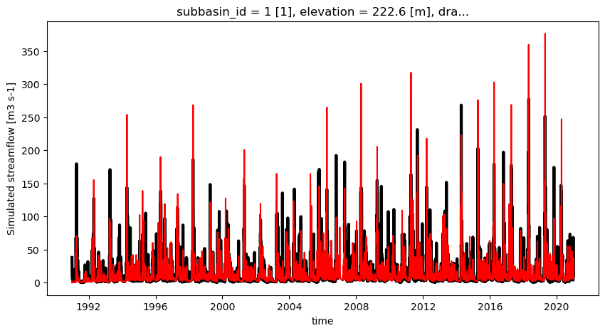
[21]:
ax = plt.figure(figsize=(10, 5))
qobs.q.plot(color="k", linewidth=3)
best_simulation.q.plot(color="r")
[21]:
[<matplotlib.lines.Line2D at 0x7f5f930e23c0>]
Calculation of hydroclimatological indicators
[22]:
import numpy as np
import xclim

import xhydro.frequency_analysis as xhfa
Non-frequential indicators
INFO
For more information on this section and available options, consult the Climate change analysis notebook.
INFO
Custom indicators in xHydro are built by following the YAML formatting required by xclim.
A custom indicator built using xclim.core.indicator.Indicator.from_dict will need these elements:
“data”: A dictionary with the following information:
“base”: The “YAML ID” obtained from here.
“input”: A dictionary linking the default xclim input to the name of your variable. Needed only if it is different. In the link above, they are the string following “Uses:”.
“parameters”: A dictionary containing all other parameters for a given indicator. In the link above, the easiest way to access them is by clicking the link in the top-right corner of the box describing a given indicator.
More entries can be used here, as described in the xclim documentation under “identifier”.
“identifier”: A custom name for your indicator. This will be the name returned in the results.
“module”: Needed, but can be anything. To prevent an accidental overwriting of
xclimindicators, it is best to use something different from: [“atmos”, “land”, “generic”].
For a climate change impact analysis, the typical process to compute non-frequential indicators would be to:
Define the indicators either through the
xclimfunctionalities shown below or through a YAML file.Call
xhydro.indicators.compute_indicators, which would produce annual results through a dictionary, where each key represents the requested frequencies.Call
xhydro.cc.climatological_opon each entry of the dictionary to compute the 30-year average.Recombine the datasets.
However, if the annual results are not required, xhydro.cc.produce_horizon can bypass steps 2 to 4 and alleviate a lot of hassle. It accomplishes that by removing the time axis and replacing it for a horizon dimension that represents a slice of time. In the case of seasonal or monthly indicators, a corresponding season or month dimension is also added.
We will compute the mean summer flow (an annual indicator) and mean monthly flows.
[23]:
indicators = [
    # Mean summer flow
    xclim.core.indicator.Indicator.from_dict(
        data={
            "base": "stats",
            "input": {"da": "q"},
            "parameters": {"op": "mean", "indexer": {"month": [6, 7, 8]}},
        },
        identifier="qmoy_summer",
        module="hydro",
    ),
    # Mean monthly flow
    xclim.core.indicator.Indicator.from_dict(
        data={
            "base": "stats",
            "input": {"da": "q"},
            "parameters": {"op": "mean", "freq": "MS"},
        },
        identifier="qmoy_monthly",
        module="hydro",
    ),
]

ds_indicators = xh.cc.produce_horizon(
    best_simulation, indicators=indicators, periods=["1991", "2020"]
)

ds_indicators
[23]:
<xarray.Dataset> Size: 316B
Dimensions:             (horizon: 1, month: 12)
Coordinates:
  * horizon             (horizon) <U9 36B '1991-2020'
  * month               (month) <U3 144B 'JAN' 'FEB' 'MAR' ... 'OCT' 'NOV' 'DEC'
    subbasin_id         <U1 4B '1'
    elevation           float32 4B 222.6
    drainage_area       float64 8B 585.6
    centroid_longitude  float64 8B -71.26
    centroid_latitude   float64 8B 46.45
Data variables:
    qmoy_summer         (horizon) float64 8B 9.589
    qmoy_monthly        (horizon, month) float64 96B 5.919 4.565 ... 12.27 9.125
Attributes:
    Conventions:           CF-1.6
    featureType:           timeSeries
    history:               Created on 2026-03-31T14:36:41 by Raven 4.1
    description:           Standard Output
    references:            Craig J.R. and the Raven Development Team Raven us...
    model_id:              GR4JCN
    Raven_version:         4.1
    RavenPy_version:       0.20.0
    cat:xrfreq:            fx
    cat:frequency:         fx
    cat:processing_level:  horizons
cat:variable: ('qmoy_monthly',)Frequency analysis
INFO
For more information on this section and available options, consult the Local frequency analysis notebook.
A frequency analysis typically follows these steps:
Get the raw data needed for the analysis, such as annual maximums, through
xhydro.indicators.get_yearly_op.Call
xhfa.local.fitto obtain the parameters for a specified number of distributions, such as Gumbel, GEV, and Pearson-III.(Optional) Call
xhfa.local.criteriato obtain goodness-of-fit parameters.Call
xhfa.local.parametric_quantilesto obtain the return levels.
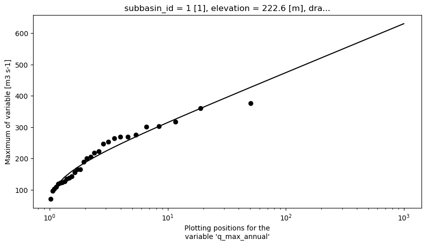
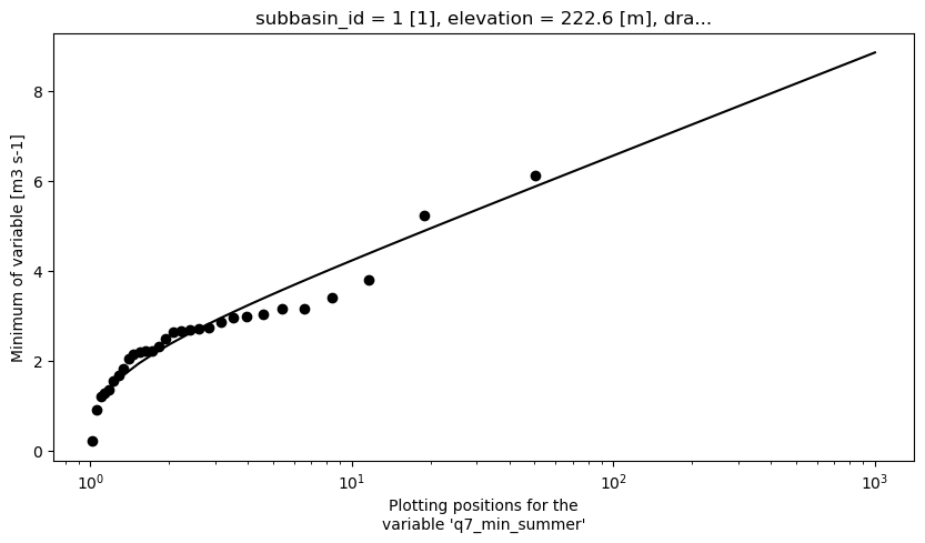
We will compute the 20 and 100-year annual maximums, as well as the 2-year minimum 7-day summer flow.
[24]:
qref_max = xh.indicators.get_yearly_op(
    best_simulation,
    op="max",
    timeargs={"annual": {}},
    missing="pct",
    missing_options={"tolerance": 0.15},
)
qref_min = xh.indicators.get_yearly_op(
    best_simulation,
    op="min",
    window=7,
    timeargs={"summer": {"date_bounds": ["05-01", "11-30"]}},
    missing="pct",
    missing_options={"tolerance": 0.15},
)
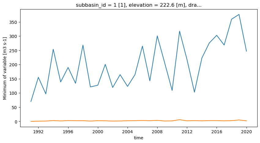
[25]:
ax = plt.figure(figsize=(10, 5))
qref_max.q_max_annual.dropna("time", how="all").plot()
qref_min.q7_min_summer.dropna("time", how="all").plot()
[25]:
[<matplotlib.lines.Line2D at 0x7f5f920e8440>]
[26]:
params_max = xhfa.local.fit(
    qref_max,
    distributions=["genextreme", "gumbel_r", "norm", "pearson3"],
    method="MLE",
    min_years=20,
).compute()
params_min = xhfa.local.fit(
    qref_min,
    distributions=["genextreme", "gumbel_r", "norm", "pearson3"],
    method="MLE",
    min_years=20,
).compute()

params_max
[26]:
<xarray.Dataset> Size: 436B
Dimensions:             (scipy_dist: 4, dparams: 4)
Coordinates:
  * scipy_dist          (scipy_dist) <U10 160B 'genextreme' ... 'pearson3'
  * dparams             (dparams) <U5 80B 'c' 'skew' 'loc' 'scale'
    horizon             <U9 36B '1991-2020'
    subbasin_id         <U1 4B '1'
    elevation           float32 4B 222.6
    drainage_area       float64 8B 585.6
    centroid_longitude  float64 8B -71.26
    centroid_latitude   float64 8B 46.45
Data variables:
    q_max_annual        (scipy_dist, dparams) float64 128B 0.08161 nan ... 87.46
Attributes: (12/13)
    Conventions:           CF-1.6
    featureType:           timeSeries
    history:               Created on 2026-03-31T14:36:41 by Raven 4.1
    description:           Standard Output
    references:            Craig J.R. and the Raven Development Team Raven us...
    model_id:              GR4JCN
    ...                    ...
    RavenPy_version:       0.20.0
    cat:xrfreq:            YS-JAN
    cat:frequency:         yr
    cat:processing_level:  indicators
    cat:variable:          ('q_max_annual',)
cat:id: While not foolproof, the best fit can be identified using the Bayesian Information Criteria.
[27]:
criteria_max = xhfa.local.criteria(qref_max, params_max)
criteria_max = str(
    criteria_max.isel(
        scipy_dist=criteria_max.q_max_annual.sel(criterion="bic").argmin(dim="scipy_dist").values
    ).scipy_dist.values
)  # Get the best fit as a string
print(f"Best distribution for the annual maxima: {criteria_max}")

criteria_min = xhfa.local.criteria(qref_min, params_min)
criteria_min = str(
    criteria_min.isel(
        scipy_dist=criteria_min.q7_min_summer.sel(criterion="bic").argmin(dim="scipy_dist").values
    ).scipy_dist.values
)  # Get the best fit as a string
print(f"Best distribution for the summer 7-day minima: {criteria_min}")
Best distribution for the annual maxima: gumbel_r
Best distribution for the summer 7-day minima: gumbel_r
Plotting functions will eventually come to xhydro.frequency_analysis, but they currently are a work-in-progress and are hidden by default. Until a public function is added to the library, they can still be called to illustrate the results.
[28]:
# Plotting
data_max = xhfa.local._prepare_plots(
    params_max, xmin=1, xmax=1000, npoints=50, log=True
)
data_max["q_max_annual"].attrs["long_name"] = "q"
pp = xhfa.local._get_plotting_positions(qref_max[["q_max_annual"]])

ax = plt.figure(figsize=(10, 5))
data_max.q_max_annual.sel(scipy_dist=criteria_max).plot(color="k")
plt.xscale("log")
pp.plot.scatter(
    x="q_max_annual_pp",
    y="q_max_annual",
    color="k",
)
[28]:
<matplotlib.collections.PathCollection at 0x7f5f920b6a50>
[29]:
# Plotting
data_min = xhfa.local._prepare_plots(
    params_min, xmin=1, xmax=1000, npoints=50, log=True
)
data_min["q7_min_summer"].attrs["long_name"] = "q"
pp = xhfa.local._get_plotting_positions(qref_min[["q7_min_summer"]])

ax = plt.figure(figsize=(10, 5))
data_min.q7_min_summer.sel(scipy_dist=criteria_min).plot(color="k")
plt.xscale("log")
pp.plot.scatter(
    x="q7_min_summer_pp",
    y="q7_min_summer",
    color="k",
)
[29]:
<matplotlib.collections.PathCollection at 0x7f5f90358690>
[30]:
# Computation of return levels
rl_max = xhfa.local.parametric_quantiles(
    params_max.sel(scipy_dist=criteria_max).expand_dims("scipy_dist"),
    return_period=[20, 100],
).squeeze()
rl_min = xhfa.local.parametric_quantiles(
    params_min.sel(scipy_dist=criteria_min).expand_dims("scipy_dist"),
    return_period=[2],
    mode="min",
).squeeze()
rl_max
[30]:
<xarray.Dataset> Size: 148B
Dimensions:             (return_period: 2)
Coordinates:
  * return_period       (return_period) int64 16B 20 100
    p_quantile          (return_period) float64 16B 0.95 0.99
    horizon             <U9 36B '1991-2020'
    scipy_dist          <U8 32B 'gumbel_r'
    subbasin_id         <U1 4B '1'
    elevation           float32 4B 222.6
    drainage_area       float64 8B 585.6
    centroid_longitude  float64 8B -71.26
    centroid_latitude   float64 8B 46.45
Data variables:
    q_max_annual        (return_period) float64 16B 363.4 473.8
Attributes: (12/13)
    Conventions:           CF-1.6
    featureType:           timeSeries
    history:               Created on 2026-03-31T14:36:41 by Raven 4.1
    description:           Standard Output
    references:            Craig J.R. and the Raven Development Team Raven us...
    model_id:              GR4JCN
    ...                    ...
    RavenPy_version:       0.20.0
    cat:xrfreq:            YS-JAN
    cat:frequency:         yr
    cat:processing_level:  indicators
    cat:variable:          ('q_max_annual',)
cat:id: [31]:
print(
    f"20-year annual maximum: {np.round(rl_max.q_max_annual.sel(return_period=20).values, 1)} m³/s"
)
print(
    f"100-year annual maximum: {np.round(rl_max.q_max_annual.sel(return_period=100).values, 1)} m³/s"
)
print(
    f"2-year minimum 7-day summer flow: {np.round(rl_min.q7_min_summer.values, 1)} m³/s"
)
20-year annual maximum: 363.4 m³/s
100-year annual maximum: 473.8 m³/s
2-year minimum 7-day summer flow: 2.4 m³/s
Future streamflow simulations and indicators
Future meteorological data
Now that we have access to a calibrated hydrological model and historical indicators, we can perform the climate change analysis. This example will use a set of CMIP6 models that have been bias adjusted using ERA5-Land, for consistency with the reference product. Specifically, we will use the ESPO-G6-E5L dataset, also hosted on PAVICS. While it is recommended to use multiple emission scenarios, this example will only use the SSP2-4.5 simulations from 14 climate models.
We can mostly reuse the same code as above. One difference is that climate models often use custom calendars. Raven can manage them, but it can still be required to convert them back to standard ones. The convert_calendar_missing argument of format_input can be used for that matter. If “True”, it will linearly interpolate temperature data and put 0 precipitation for calendar days that are being added to the dataset.
[32]:
models = [
    "day_ESPO-G6-E5L_v1.0.0_CMIP6_ScenarioMIP_NAM_CAS_FGOALS-g3_ssp245_r1i1p1f1_1950-2100.ncml",
    "day_ESPO-G6-E5L_v1.0.0_CMIP6_ScenarioMIP_NAM_CMCC_CMCC-ESM2_ssp245_r1i1p1f1_1950-2100.ncml",
    "day_ESPO-G6-E5L_v1.0.0_CMIP6_ScenarioMIP_NAM_CSIRO-ARCCSS_ACCESS-CM2_ssp245_r1i1p1f1_1950-2100.ncml",
    "day_ESPO-G6-E5L_v1.0.0_CMIP6_ScenarioMIP_NAM_CSIRO_ACCESS-ESM1-5_ssp245_r1i1p1f1_1950-2100.ncml",
    "day_ESPO-G6-E5L_v1.0.0_CMIP6_ScenarioMIP_NAM_DKRZ_MPI-ESM1-2-HR_ssp245_r1i1p1f1_1950-2100.ncml",
    "day_ESPO-G6-E5L_v1.0.0_CMIP6_ScenarioMIP_NAM_INM_INM-CM5-0_ssp245_r1i1p1f1_1950-2100.ncml",
    "day_ESPO-G6-E5L_v1.0.0_CMIP6_ScenarioMIP_NAM_MIROC_MIROC6_ssp245_r1i1p1f1_1950-2100.ncml",
    "day_ESPO-G6-E5L_v1.0.0_CMIP6_ScenarioMIP_NAM_MPI-M_MPI-ESM1-2-LR_ssp245_r1i1p1f1_1950-2100.ncml",
    "day_ESPO-G6-E5L_v1.0.0_CMIP6_ScenarioMIP_NAM_MRI_MRI-ESM2-0_ssp245_r1i1p1f1_1950-2100.ncml",
    "day_ESPO-G6-E5L_v1.0.0_CMIP6_ScenarioMIP_NAM_NCC_NorESM2-LM_ssp245_r1i1p1f1_1950-2100.ncml",
    "day_ESPO-G6-E5L_v1.0.0_CMIP6_ScenarioMIP_NAM_CNRM-CERFACS_CNRM-ESM2-1_ssp245_r1i1p1f2_1950-2100.ncml",
    "day_ESPO-G6-E5L_v1.0.0_CMIP6_ScenarioMIP_NAM_NIMS-KMA_KACE-1-0-G_ssp245_r1i1p1f1_1950-2100.ncml",
    "day_ESPO-G6-E5L_v1.0.0_CMIP6_ScenarioMIP_NAM_NOAA-GFDL_GFDL-ESM4_ssp245_r1i1p1f1_1950-2100.ncml",
    "day_ESPO-G6-E5L_v1.0.0_CMIP6_ScenarioMIP_NAM_BCC_BCC-CSM2-MR_ssp245_r1i1p1f1_1950-2100.ncml",
]
The code below will showcase how to proceed with the first simulation, but it could be looped to process all 14.
[33]:
model = models[0]

meteo_sim = xr.open_dataset(
    f"https://pavics.ouranos.ca/twitcher/ows/proxy/thredds/dodsC/datasets/simulations/bias_adjusted/cmip6/ouranos/ESPO-G/ESPO-G6-E5Lv1.0.0/{model}",
    engine="netcdf4",
    chunks={"time": 365, "lon": 50, "lat": 50},
)
meteo_sim = xscen.spatial.subset(meteo_sim, method="shape", tile_buffer=2, shape=gdf)
# Add altitude data
meteo_sim = meteo_sim.assign_coords(
    {"elevation": xr.ones_like(meteo_sim.pr.isel(time=0).drop_vars("time")) * 350}
)
meteo_sim["elevation"].attrs = {"units": "m"}

# Format the dataset
meteo_sim, config_meteo_sim = xh.modelling.format_input(
    meteo_sim,
    model="GR4JCN",
    convert_calendar_missing=True,
    save_as=notebook_folder / "_data" / f"meteo_sim0.nc",
)
Future streamflow data and indicators
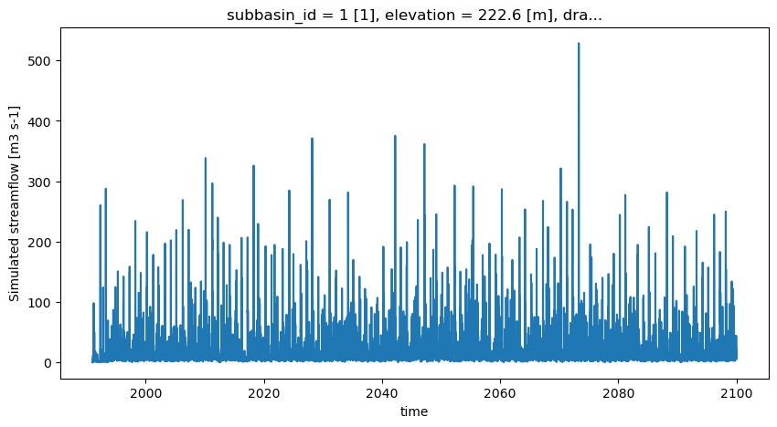
Once again, the same code as before can be roughly reused here, but with xhydro.modelling.hydrological_model. The main difference is that the best parameters can be used when setting up the hydrological model, and that the dates are the full range going to 2100.
Indicators are also computed similarly, with the addition of using a list of periods in the periods argument to create a horizon dimension, instead of a single period. The xhydro.frequency_analysis.fit function can also accept a periods argument.
The code below will once again only showcase the first simulation, but could be used to process all 14.
[34]:
from copy import deepcopy

import xhydro.modelling as xhm
[35]:
model_cfg = (
    deepcopy(model_config) | config_meteo_sim
)  # Update the config with the new information from the simulation file
model_cfg["parameters"] = np.array(best_parameters)
model_cfg["start_date"] = "1991-01-01"
model_cfg["end_date"] = "2099-12-31"

qsim = xhm.hydrological_model(model_cfg).run()
[36]:
plt.figure(figsize=(10, 5))
qsim.q.plot()
[36]:
[<matplotlib.lines.Line2D at 0x7f5f906d7e00>]
[37]:
# Non-frequential indicators
ds_indicators = xh.cc.produce_horizon(
    qsim, indicators=indicators, periods=[["1991", "2020"], ["2070", "2099"]]
)

# Frequency analysis
qsim_max = xh.indicators.get_yearly_op(
    qsim,
    op="max",
    timeargs={"annual": {}},
    missing="pct",
    missing_options={"tolerance": 0.15},
)
qsim_min = xh.indicators.get_yearly_op(
    qsim,
    op="min",
    window=7,
    timeargs={"summer": {"date_bounds": ["05-01", "11-30"]}},
    missing="pct",
    missing_options={"tolerance": 0.15},
)

params_max = xhfa.local.fit(
    qsim_max,
    distributions=["genextreme", "gumbel_r", "norm", "pearson3"],
    method="MLE",
    min_years=20,
    periods=[["1991", "2020"], ["2070", "2099"]],
).compute()
params_min = xhfa.local.fit(
    qsim_min,
    distributions=["genextreme", "gumbel_r", "norm", "pearson3"],
    method="MLE",
    min_years=20,
    periods=[["1991", "2020"], ["2070", "2099"]],
).compute()

criteria_max = xhfa.local.criteria(
    qsim_max.sel(time=slice("1991", "2020")), params_max.sel(horizon="1991-2020")
)
criteria_max = str(
    criteria_max.isel(
        scipy_dist=criteria_max.q_max_annual.sel(criterion="bic").argmin(dim="scipy_dist").values
    ).scipy_dist.values
)  # Get the best fit as a string

criteria_min = xhfa.local.criteria(
    qsim_min.sel(time=slice("1991", "2020")), params_min.sel(horizon="1991-2020")
)
criteria_min = str(
    criteria_min.isel(
        scipy_dist=criteria_min.q7_min_summer.sel(criterion="bic").argmin(dim="scipy_dist").values
    ).scipy_dist.values
)  # Get the best fit as a string

# Computation of return levels
rl_max = xhfa.local.parametric_quantiles(
    params_max.sel(scipy_dist=criteria_max).expand_dims("scipy_dist"),
    return_period=[20, 100],
).squeeze()
rl_min = xhfa.local.parametric_quantiles(
    params_min.sel(scipy_dist=criteria_min).expand_dims("scipy_dist"),
    return_period=[2],
    mode="min",
).squeeze()

# Combine all indicators
ds_indicators = xr.merge([ds_indicators, rl_max, rl_min], compat="override")

ds_indicators
[37]:
<xarray.Dataset> Size: 568B
Dimensions:             (horizon: 2, month: 12, return_period: 2)
Coordinates:
  * horizon             (horizon) <U9 72B '1991-2020' '2070-2099'
  * month               (month) <U3 144B 'JAN' 'FEB' 'MAR' ... 'OCT' 'NOV' 'DEC'
  * return_period       (return_period) int64 16B 20 100
    p_quantile          (return_period) float64 16B 0.95 0.99
    subbasin_id         <U1 4B '1'
    elevation           float32 4B 222.6
    drainage_area       float64 8B 585.6
    centroid_longitude  float64 8B -71.26
    centroid_latitude   float64 8B 46.45
    scipy_dist          <U8 32B 'gumbel_r'
Data variables:
    qmoy_summer         (horizon) float64 16B 9.707 8.611
    qmoy_monthly        (horizon, month) float64 192B 7.359 6.124 ... 11.74
    q_max_annual        (return_period, horizon) float64 32B 325.4 ... 437.9
    q7_min_summer       (horizon) float64 16B 2.109 1.983
Attributes:
    Conventions:           CF-1.6
    featureType:           timeSeries
    history:               Created on 2026-03-31T14:40:01 by Raven 4.1
    description:           Standard Output
    references:            Craig J.R. and the Raven Development Team Raven us...
    model_id:              GR4JCN
    Raven_version:         4.1
    RavenPy_version:       0.20.0
    cat:xrfreq:            fx
    cat:frequency:         fx
    cat:processing_level:  horizons
cat:variable: ('qmoy_monthly',)Climate change impacts
INFO
For more information on this section and available options, consult the Climate change analysis notebook.
This example will keep the climate change analysis fairly simple.
Compute the difference between the future and reference periods using
xhydro.cc.compute_deltas.Use those differences to compute ensemble statistics using
xhydro.cc.ensemble_stats: ensemble percentiles and agreement between the climate models.
[38]:
# Differences
deltas = xh.cc.compute_deltas(
    ds_indicators, reference_horizon="1991-2020", kind="%", rename_variables=False
).isel(horizon=-1)

# Save the results
deltas.to_netcdf(notebook_folder / "_data" / f"deltas_sim0.nc")

deltas.squeeze()
[38]:
<xarray.Dataset> Size: 404B
Dimensions:             (month: 12, return_period: 2)
Coordinates:
  * month               (month) <U3 144B 'JAN' 'FEB' 'MAR' ... 'OCT' 'NOV' 'DEC'
  * return_period       (return_period) int64 16B 20 100
    p_quantile          (return_period) float64 16B 0.95 0.99
    subbasin_id         <U1 4B '1'
    elevation           float32 4B 222.6
    drainage_area       float64 8B 585.6
    centroid_longitude  float64 8B -71.26
    centroid_latitude   float64 8B 46.45
    horizon             <U9 36B '2070-2099'
    scipy_dist          <U8 32B 'gumbel_r'
Data variables:
    qmoy_summer         float64 8B -11.29
    qmoy_monthly        (month) float64 96B 14.88 10.29 61.14 ... 22.37 24.68
    q_max_annual        (return_period) float64 16B 4.637 7.371
    q7_min_summer       float64 8B -5.966
Attributes:
    Conventions:           CF-1.6
    featureType:           timeSeries
    history:               Created on 2026-03-31T14:40:01 by Raven 4.1
    description:           Standard Output
    references:            Craig J.R. and the Raven Development Team Raven us...
    model_id:              GR4JCN
    Raven_version:         4.1
    RavenPy_version:       0.20.0
    cat:xrfreq:            fx
    cat:frequency:         fx
    cat:processing_level:  deltas
cat:variable: ('qmoy_monthly',)There are many ways to create the ensemble itself. If using a dictionary of datasets, the key will be used to name each element of the new realization dimension. This can be very useful when performing more detailed analyses or when wanting to weight the different models based, for example, on the number of available simulations. In our case, since we only wish to compute ensemble statistics, we can keep it simpler and provide a list.
[39]:
import pooch

# Acquire deltas for the other 13 simulations
from xhydro.testing.helpers import (  # In-house function to access xhydro-testdata
    deveraux,
)

deltas_files = deveraux().fetch("use_case/deltas.zip", processor=pooch.Unzip())
deltas_files = xclim.ensembles.create_ensemble(deltas_files)

# Fix variable names and combine with the file we just created
deltas_files = deltas_files.rename(
    {"streamflow_max_annual": "q_max_annual", "streamflow7_min_summer": "q7_min_summer"}
)
deltas_sim0 = xr.open_dataset(
    notebook_folder / "_data" / f"deltas_sim0.nc"
).assign_coords({"realization": 13})
deltas_files = xr.concat([deltas_files, deltas_sim0], dim="realization")
clear_output(wait=False)
[40]:
# Statistics to compute
statistics = {
    "ensemble_percentiles": {"values": [10, 25, 50, 75, 90], "split": False},
    "robustness_fractions": {"test": None},
}

ens_stats = xh.cc.ensemble_stats(deltas_files, statistics)

ens_stats
[40]:
<xarray.Dataset> Size: 2kB
Dimensions:                         (percentiles: 5, month: 12, return_period: 2)
Coordinates:
  * percentiles                     (percentiles) int64 40B 10 25 50 75 90
  * month                           (month) <U3 144B 'JAN' 'FEB' ... 'NOV' 'DEC'
  * return_period                   (return_period) int64 16B 20 100
    p_quantile                      (return_period) float64 16B 0.95 0.99
    basin_name                      <U7 28B 'sub_001'
    horizon                         <U9 36B '2070-2099'
    subbasin_id                     <U1 4B '1'
    elevation                       float32 4B 222.6
    drainage_area                   float64 8B 585.6
    centroid_longitude              float64 8B -71.26
    centroid_latitude               float64 8B 46.45
Data variables: (12/32)
    qmoy_summer                     (percentiles) float64 40B -14.0 ... 19.14
    qmoy_monthly                    (month, percentiles) float64 480B dask.array<chunksize=(12, 5), meta=np.ndarray>
    q_max_annual                    (return_period, percentiles) float64 80B dask.array<chunksize=(2, 5), meta=np.ndarray>
    q7_min_summer                   (percentiles) float64 40B -28.54 ... 11.68
    qmoy_summer_changed             float64 8B 1.0
    qmoy_summer_positive            float64 8B 0.5714
    ...                              ...
    q7_min_summer_positive          float64 8B 0.2143
    q7_min_summer_changed_positive  float64 8B 0.2143
    q7_min_summer_negative          float64 8B 0.7857
    q7_min_summer_changed_negative  float64 8B 0.7857
    q7_min_summer_valid             float64 8B 1.0
    q7_min_summer_agree             float64 8B 0.7857
Attributes:
    cat:xrfreq:            fx
    cat:frequency:         fx
    cat:processing_level:  ensemble
    cat:variable:          qmoy_monthly
ensemble_size: 4[41]:
# Recreate the boxplots based on the computed percentiles
fig, axes = plt.subplots(nrows=1, ncols=3, figsize=(13, 5), sharey=True)

ax = plt.subplot(1, 3, 1)
for i, rp in enumerate(ens_stats.return_period.values):
    stats = [
        {
            "label": rp,
            "med": ens_stats.q_max_annual.sel(percentiles=50, return_period=rp).values,
            "q1": ens_stats.q_max_annual.sel(percentiles=25, return_period=rp).values,
            "q3": ens_stats.q_max_annual.sel(percentiles=75, return_period=rp).values,
            "whislo": ens_stats.q_max_annual.sel(
                percentiles=10, return_period=rp
            ).values,
            "whishi": ens_stats.q_max_annual.sel(
                percentiles=90, return_period=rp
            ).values,
        }
    ]

    ax.bxp(stats, showfliers=False, positions=[i], widths=0.5)
ax.set_title("Maximum annual streamflow")
plt.xlabel("Return period")
plt.ylabel("Difference Fut-Hist (%)")

ax = plt.subplot(1, 3, 2)
for i, rp in enumerate(ens_stats.return_period.values):
    stats = [
        {
            "label": rp,
            "med": ens_stats.q7_min_summer.sel(percentiles=50).values,
            "q1": ens_stats.q7_min_summer.sel(percentiles=25).values,
            "q3": ens_stats.q7_min_summer.sel(percentiles=75).values,
            "whislo": ens_stats.q7_min_summer.sel(percentiles=10).values,
            "whishi": ens_stats.q7_min_summer.sel(percentiles=90).values,
        }
    ]

    ax.bxp(stats, showfliers=False, positions=[i], widths=0.5)
ax.set_title("Minimum summer streamflow (7-day avg)")
plt.xlabel("")

ax = plt.subplot(1, 3, 3)
stats = [
    {
        "label": "",
        "med": ens_stats.qmoy_summer.sel(percentiles=50).values,
        "q1": ens_stats.qmoy_summer.sel(percentiles=25).values,
        "q3": ens_stats.qmoy_summer.sel(percentiles=75).values,
        "whislo": ens_stats.qmoy_summer.sel(percentiles=10).values,
        "whishi": ens_stats.qmoy_summer.sel(percentiles=90).values,
    }
]

ax.bxp(stats, showfliers=False, positions=[i], widths=0.25)
ax.set_title("Mean summer flow")

plt.show()
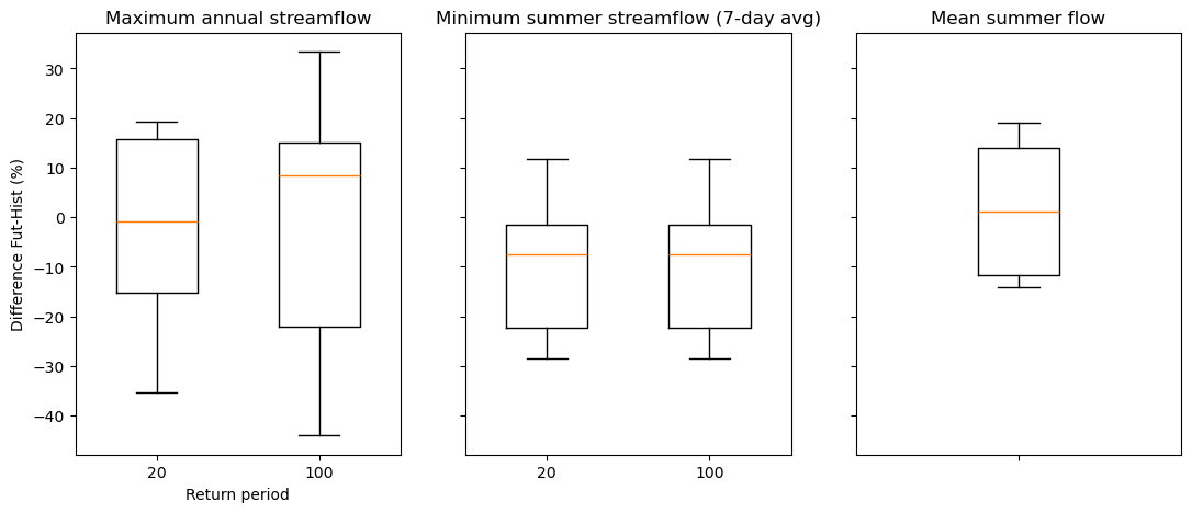
[42]:
print(
    f"Fraction of simulations with a positive change (maximum streamflow): {ens_stats.q_max_annual_positive.values}"
)
print(
    f"Fraction of simulations with a positive change (minimum summer streamflow): {ens_stats.q7_min_summer_positive.values}"
)
print(
    f"Fraction of simulations with a positive change (mean summer streamflow): {ens_stats.qmoy_summer_positive.values}"
)
Fraction of simulations with a positive change (maximum streamflow): [0.5        0.64285714]
Fraction of simulations with a positive change (minimum summer streamflow): 0.21428571428571427
Fraction of simulations with a positive change (mean summer streamflow): 0.5714285714285714