9. Inputs for the Probable Maximum flood (PMF)
9.1. Probable Maximum Precipitation (PMP)
Probable Maximum Precipitation (PMP) is the theoretical maximum amount of precipitation that could occur at a specific location within a given period of time, considering the most extreme meteorological conditions. PMP is a critical parameter in hydrology, especially for the design of infrastructure such as dams, reservoirs, and drainage systems.
There are several methods for calculating PMP, each varying in complexity and the type of data used. The method currently implemented in xHydro is based on the approach outlined by Clavet-Gaumont et al. (2017). This method involves maximizing the precipitable water over a given location, which refers to the total water vapor in the atmosphere that could potentially be converted into precipitation under ideal conditions. By maximizing this
value, the method estimates the maximum precipitation that could theoretically occur at the location.
[1]:
from pathlib import Path

import hvplot.xarray
import matplotlib.pyplot as plt
import numpy as np
import pooch
import xarray as xr
import xclim

import xhydro as xh
from xhydro.testing.helpers import deveraux
ERROR 1: PROJ: proj_create_from_database: Open of /home/docs/checkouts/readthedocs.org/user_builds/xhydro/conda/stable/share/proj failed
/home/docs/checkouts/readthedocs.org/user_builds/xhydro/conda/stable/lib/python3.14/site-packages/xhydro/__init__.py:21: UserWarning: The `exactextract` library is not present in the environment and will not be used.
9.1.1. Acquiring data
The acquisition of climatological data is outside the scope of xHydro. However, some examples of how to obtain and handle such data are provided in the GIS operations and Use Case Example notebooks. For this notebook, we will use a test dataset consisting of 2 years and 3x3 grid cells from CanESM5 climate model data. In a real application, it would be preferable to have as many years of data as possible.
To perform the analysis, certain climatological variables are required.
Daily Timestep Variables:
pr→ Precipitation fluxsnw→ Snow water equivalenthus→ Specific humidity for multiple pressure levelszg→ Geopotential height for multiple pressure levels
Fixed Field Variables:
orog→ Surface altitude
In cold regions, it may be necessary to split total precipitation into rainfall and snowfall components. Many climate models already provide this data separately. However, if this data is not directly available, libraries such as xclim can approximate the split using precipitation and temperature data.
[2]:
from pathlib import Path

import xhydro as xh

path_day_zip = deveraux().fetch(
    "pmp/CMIP.CCCma.CanESM5.historical.r1i1p1f1.day.gn.zarr.zip",
    pooch.Unzip(),
)
ds_day = xr.open_zarr(Path(path_day_zip[0]).parents[0])

path_fx_zip = deveraux().fetch(
    "pmp/CMIP.CCCma.CanESM5.historical.r1i1p1f1.fx.gn.zarr.zip",
    pooch.Unzip(),
)
ds_fx = xr.open_zarr(Path(path_fx_zip[0]).parents[0])

# There are a few issues with attributes in this dataset that we need to address
ds_day["pr"].attrs = {"units": "mm", "long_name": "precipitation"}
ds_day["prsn"].attrs = {"units": "mm", "long_name": "snowfall"}
ds_day["rf"].attrs = {"units": "mm", "long_name": "rainfall"}

# Combine both datasets
ds = ds_day.convert_calendar("standard")
ds["orog"] = ds_fx["orog"]
ds
[2]:
<xarray.Dataset> Size: 643kB
Dimensions:      (time: 730, plev: 8, y: 3, x: 3)
Coordinates:
  * time         (time) datetime64[ns] 6kB 2010-01-01T12:00:00 ... 2011-12-31...
  * plev         (plev) float64 64B 1e+05 8.5e+04 7e+04 ... 1e+04 5e+03 1e+03
  * y            (y) float64 24B 43.25 46.04 48.84
  * x            (x) float64 24B 281.2 284.1 286.9
    height       float64 8B ...
Data variables:
    hus          (time, plev, y, x) float32 210kB dask.array<chunksize=(214, 8, 3, 3), meta=np.ndarray>
    lat_bounds   (y) float64 24B dask.array<chunksize=(3,), meta=np.ndarray>
    lon_bounds   (x) float64 24B dask.array<chunksize=(3,), meta=np.ndarray>
    pr           (time, y, x) float64 53kB dask.array<chunksize=(730, 3, 3), meta=np.ndarray>
    prsn         (time, y, x) float64 53kB dask.array<chunksize=(730, 3, 3), meta=np.ndarray>
    rf           (time, y, x) float64 53kB dask.array<chunksize=(730, 3, 3), meta=np.ndarray>
    snw          (time, y, x) float32 26kB dask.array<chunksize=(730, 3, 3), meta=np.ndarray>
    tas          (time, y, x) float32 26kB dask.array<chunksize=(730, 3, 3), meta=np.ndarray>
    time_bounds  (time) object 6kB dask.array<chunksize=(730,), meta=np.ndarray>
    zg           (time, plev, y, x) float32 210kB dask.array<chunksize=(239, 8, 3, 3), meta=np.ndarray>
    orog         (y, x) float32 36B dask.array<chunksize=(3, 3), meta=np.ndarray>
Attributes: (12/56)
    CCCma_model_hash:            3dedf95315d603326fde4f5340dc0519d80d10c0
    CCCma_parent_runid:          rc3-pictrl
    CCCma_pycmor_hash:           33c30511acc319a98240633965a04ca99c26427e
    CCCma_runid:                 rc3.1-his01
    Conventions:                 CF-1.7 CMIP-6.2
    YMDH_branch_time_in_child:   1850:01:01:00
    ...                          ...
    title:                       CanESM5 output prepared for CMIP6
    tracking_id:                 hdl:21.14100/d0a84c86-7fb1-4de4-8837-574504c...
    variable_id:                 hus
    variant_label:               r1i1p1f1
    version:                     v20190429
version_id: v201904299.1.2. Computing the PMP
The method outlined by Clavet-Gaumont et al. (2017) follows these steps:
- Identification of Major Precipitation Events:The first step involves identifying the major precipitation events that will be maximized. This is done by filtering events based on a specified threshold.
- Computation of Monthly 100-Year Precipitable Water:The next step involves calculating the 100-year precipitable water on a monthly basis using the Generalized Extreme Value (GEV) distribution, with a maximum cap of 20% greater than the largest observed value.
- Maximization of Precipitation During Events:In this step, the precipitation events are maximized based on the ratio between the 100-year monthly precipitable water and the precipitable water during the major precipitation events. In snow-free regions, this is the final result.
- Seasonal Separation in Cold Regions:In cold regions, the results are separated into seasons (e.g., spring, summer) to account for snow during the computation of Probable Maximum Floods (PMF).
This method provides a comprehensive approach for estimating the PMP, taking into account both temperature and precipitation variations across different regions and seasons.
9.1.3. Major precipitation events
The first step in calculating the Probable Maximum Precipitation (PMP) involves filtering the precipitation data to retain only the events that exceed a certain threshold. These major precipitation events will be maximized in subsequent steps. The function xh.indicators.pmp.major_precipitation_events can be used for this purpose. It also provides the option to sum precipitation over a specified number of days, which can help aggregate storm events. For 2D data, such as in this example, each
grid point is treated independently.
In this example, we will filter out the 10% most intense storms to avoid overemphasizing smaller precipitation events during the maximization process. Additionally, we will focus on rainfall (rf) rather than total precipitation (pr) to exclude snowstorms and ensure that we are only considering liquid precipitation events.
[3]:
Help on function major_precipitation_events in module xhydro.indicators.pmp:

major_precipitation_events(
    da: xr.DataArray,
    *,
    windows: list[int],
    quantile: float | None = None,
    min_prec: str = '0 mm'
)
    Get precipitation events that exceed a given quantile for a given time step accumulation. Based on Clavet-Gaumont et al. (2017).

    Parameters
    ----------
    da : xr.DataArray
        DataArray containing the precipitation values.
    windows : list of int
        List of the number of time steps to accumulate precipitation.
    quantile : float, optional
        Threshold that limits the events to those that exceed this quantile.
        If `quantile` is None, the function returns all the accumulated values.
    min_prec : Quantified
        Minimum precipitation value to consider an event.
        Values equal to `min_prec` are excluded. Defaults to 0 mm.

    Returns
    -------
    xr.DataArray
        Masked DataArray containing the major precipitation events.

    Notes
    -----
    https://doi.org/10.1016/j.ejrh.2017.07.003
[4]:
precipitation_events = xh.indicators.pmp.major_precipitation_events(
    ds.rf, windows=[1], quantile=0.9, min_prec="0.1 mm"
)

ds.rf.isel(x=1, y=1).hvplot() * precipitation_events.isel(
    x=1, y=1, window=0
).hvplot.scatter(color="red")
[4]:
9.1.4. Daily precipitable water
WARNING
This step should be avoided if possible, as it involves approximating precipitable water from the integral of specific humidity and will be highly sensitive to the number of pressure levels used. If available, users are strongly encouraged to use a variable or combination of variables that directly represent precipitable water.
Precipitable water can be estimated using xhydro.indicators.pmp.precipitable_water by integrating the vertical column of humidity. This process requires specific humidity, geopotential height, and elevation data. The resulting value represents the total amount of water vapor that could potentially be precipitated from the atmosphere under ideal conditions.
[5]:
Help on function precipitable_water in module xhydro.indicators.pmp:

precipitable_water(
    *,
    hus: xr.DataArray,
    zg: xr.DataArray,
    orog: xr.DataArray,
    windows: list[int] | None = None,
    beta_func: bool = True,
    add_pre_lay: bool = False
)
    Compute precipitable water based on Clavet-Gaumont et al. (2017) and Rousseau et al (2014).

    Parameters
    ----------
    hus : xr.DataArray
        Specific humidity. Must have a pressure level (plev) dimension.
    zg : xr.DataArray
        Geopotential height. Must have a pressure level (plev) dimension.
    orog : xr.DataArray
        Surface altitude.
    windows : list of int, optional
        Duration of the event in time steps. Defaults to [1].
        Note that an additional time step will be added to the window size to account for antecedent conditions.
    beta_func : bool, optional
        If True, use the beta function proposed by Boer (1982) to get the pressure layers above the topography.
        If False, the surface altitude is used as the lower boundary of the atmosphere assuming that the surface altitude
        and the geopotential height are virtually identical at low altitudes.
    add_pre_lay : bool, optional
        If True, add the pressure layer between the surface and the lowest pressure level (e.g., at sea level).
        If False, only the pressure layers between the lowest and highest pressure level are considered.

    Returns
    -------
    xr.DataArray
        Precipitable water.

    Notes
    -----
    1) The precipitable water of an event is defined as the maximum precipitable water found during the entire duration of the event,
    extending up to one time step before the start of the event. Thus, the rolling operation made using `windows` is a maximum, not a sum.

    2) beta_func = True and add_pre_lay = False follow Clavet-Gaumont et al. (2017) and Rousseau et al (2014).

    3) https://doi.org/10.1016/j.ejrh.2017.07.003
       https://doi.org/10.1016/j.jhydrol.2014.10.053
       https://doi.org/10.1175/1520-0493(1982)110<1801:DEIIC>2.0.CO;2
[6]:
pw = xh.indicators.pmp.precipitable_water(
    hus=ds.hus,
    zg=ds.zg,
    orog=ds.orog,
    windows=[1],
    add_pre_lay=False,
)

pw.isel(x=1, y=1, window=0).hvplot()
[6]:
9.1.5. Monthly 100-year precipitable water
According to Clavet-Gaumont et al. (2017), a monthly 100-year precipitable water must be computed using the Generalized Extreme Value (GEV) distribution. The value should be limited to a maximum of 20% greater than the largest observed precipitable water value for a given month. This approach ensures that the estimated 100-year event is realistic and constrained by observed data.
To compute this, you can use the xh.indicators.pmp.precipitable_water_100y function. If using rebuild_time, the output will have the same time axis as the original data.
[7]:
Help on function precipitable_water_100y in module xhydro.indicators.pmp:

precipitable_water_100y(
    pw: xr.DataArray,
    *,
    dist: str,
    method: str,
    mf: float | None = None,
    n: int | None = None,
    rebuild_time: bool = True
)
    Compute the 100-year return period of precipitable water for each month. Based on Clavet-Gaumont et al. (2017).

    Parameters
    ----------
    pw : xr.DataArray
        DataArray containing the precipitable water.
    dist : str
        Probability distributions.
    method : {"ML" or "MLE", "MM", "PWM", "APP"}
        Fitting method, either maximum likelihood (ML or MLE), method of moments (MM) or approximate method (APP).
        Can also be the probability weighted moments (PWM), also called L-Moments, if a compatible `dist` object is passed.
    mf : float, optional
        Maximum majoration factor of the 100-year event compared to the maximum of the timeseries.
        Used as an upper limit for the frequency analysis.
    n : int, optional
        Minimum number of data points for each month required to fit the statistical distribution.
        If a given month contains fewer data points than this value, `pw100` is set to the maximum value of `pw` for that month.
    rebuild_time : bool
        Whether or not to reconstruct a timeseries with the same time dimensions as `pw`.

    Returns
    -------
    xr.DataArray
        Precipitable water for a 100-year return period.

    Notes
    -----
    https://doi.org/10.1016/j.ejrh.2017.07.003
[8]:
pw100 = xh.indicators.pmp.precipitable_water_100y(
    pw.sel(window=1).chunk(dict(time=-1)),
    dist="genextreme",
    method="ML",
    mf=0.2,
    rebuild_time=True,
).compute()

pw.isel(x=1, y=1, window=0).hvplot() * pw100.isel(x=1, y=1).hvplot()
[8]:
[9]:
x = np.array([2, 5, 6, 7, 7])
y = [5, 7]

np.isin(x, y)
[9]:
array([False, True, False, True, True])
9.1.6. Maximized precipitation
INFO
This step follows the methodology described in Clavet-Gaumont et al., 2017. It is referred to as “Maximizing precipitation”, however, it effectively applies a ratio based on the monthly 100-year precipitable water. If a historical event surpassed this value—such as the case observed for January 2011—the result may actually lower the precipitation, rather than increasing it.
With the information gathered so far, we can now proceed to maximize the precipitation events. Although xHydro does not provide an explicit function for this step, it can be accomplished by following these steps:
Compute the Ratio: First, calculate the ratio between the 100-year monthly precipitable water and the precipitable water during the major precipitation events.
Apply the Ratio: Next, apply this ratio to the precipitation values themselves to maximize the precipitation events accordingly.
This process effectively scales the precipitation events based on the 100-year precipitable water, giving an estimate of the maximum possible rainfall.
[10]:
# Precipitable water on the day of the major precipitation events.
pw_events = pw.where(precipitation_events > 0)
ratio = pw100 / pw_events

# Apply the ratio onto precipitation itself
precipitation_max = ratio * precipitation_events
precipitation_max.name = "maximized_precipitation"

ds.rf.isel(x=1, y=1).hvplot() * precipitation_max.isel(
    x=1, y=1, window=0
).hvplot.scatter(color="red")
[10]:
9.1.7. Seasonal Mask
In cold regions, computing Probable Maximum Floods (PMFs) often involves scenarios that combine both rainfall and snowpack. Therefore, PMP values may need to be separated into two categories: rain-on-snow (i.e., “spring”) and snow-free rainfall (i.e., “summer”).
This can be computed easily using xhydro.indicators.pmp.compute_spring_and_summer_mask, which defines the start and end dates of spring, summer, and winter based on the presence of snow on the ground, with the following criteria:
Winter:
Winter start: The first day after which there are at least 14 consecutive days with snow on the ground.
Winter end: The last day with snow on the ground, followed by at least 45 consecutive snow-free days.
Spring:
Spring start: 60 days before the end of winter.
Spring end: 30 days after the end of winter.
Summer:
The summer period is defined as the time between winters. This period is not influenced by whether it falls in the traditional summer or fall seasons, but rather simply marks the interval between snow seasons.
[11]:
Help on function compute_spring_and_summer_mask in module xhydro.indicators.pmp:

compute_spring_and_summer_mask(
    snw: xr.DataArray,
    *,
    thresh: str = '1 cm',
    window_wint_start: int = 14,
    window_wint_end: int = 45,
    spr_start: int = 60,
    spr_end: int = 30,
    freq: str = 'YS-JUL'
)
    Create a mask that defines the spring and summer seasons based on the snow water equivalent.

    Parameters
    ----------
    snw : xarray.DataArray
        Snow water equivalent. Must be a length (e.g. "mm") or a mass (e.g. "kg m-2").
    thresh : Quantified
        Threshold snow thickness to define the start and end of winter.
    window_wint_start : int
        Minimum number of days with snow depth above or equal to threshold to define the start of winter.
    window_wint_end : int
        Maximum number of days with snow depth below or equal to threshold to define the end of winter.
    spr_start : int
        Number of days before the end of winter to define the start of spring.
    spr_end : int
        Number of days after the end of winter to define the end of spring.
    freq : str
        Frequency of the time axis (annual frequency). Defaults to "YS-JUL".

    Returns
    -------
    xr.Dataset
        Dataset with two DataArrays (mask_spring and mask_summer), with values of 1 where the
        spring and summer criteria are met and 0 where they are not.
[12]:
mask = xh.indicators.pmp.compute_spring_and_summer_mask(
    ds.snw,
    thresh="1 cm",
    window_wint_end=14,  # Since the dataset used does not have a lot of snow, we need to be more lenient
    freq="YS-SEP",
)

mask
[12]:
<xarray.Dataset> Size: 111kB
Dimensions:      (time: 730, y: 3, x: 3)
Coordinates:
  * time         (time) datetime64[ns] 6kB 2010-01-01T12:00:00 ... 2011-12-31...
  * y            (y) float64 24B 43.25 46.04 48.84
  * x            (x) float64 24B 281.2 284.1 286.9
    height       float64 8B 2.0
Data variables:
    mask_spring  (time, y, x) float64 53kB dask.array<chunksize=(365, 3, 3), meta=np.ndarray>
mask_summer (time, y, x) float64 53kB dask.array<chunksize=(365, 3, 3), meta=np.ndarray>[13]:
xclim.core.units.convert_units_to(
    ds.isel(x=1, y=1).snw, "cm", context="hydro"
).hvplot() * (mask.mask_spring.isel(x=1, y=1) * 10).hvplot() * (
    mask.mask_summer.isel(x=1, y=1) * 8
).hvplot()
[13]:
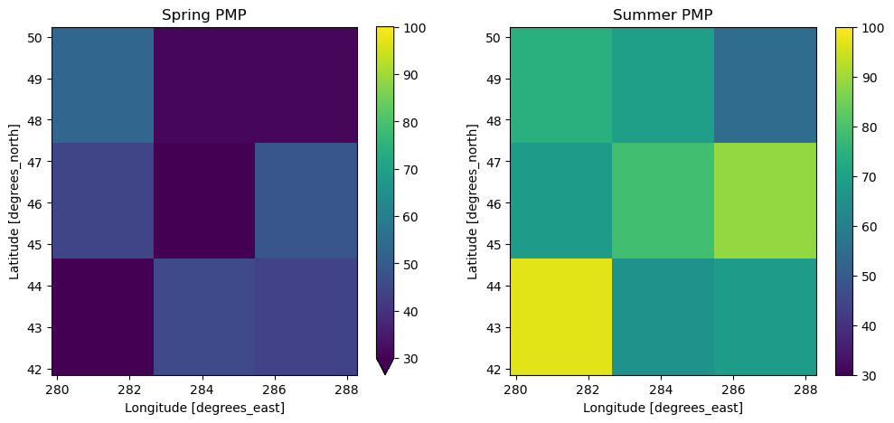
9.1.8. Final PMP
The final PMP is obtained by finding the maximum value over the time dimension. In our case, since we computed a season mask, we can further refine the results into a spring and summer PMP.
[14]:
pmp_spring = (precipitation_max * mask.mask_spring).max("time").compute()
pmp_summer = (precipitation_max * mask.mask_summer).max("time").compute()
[15]:
plt.subplots(1, 2, figsize=[12, 5])

ax = plt.subplot(1, 2, 1)
pmp_spring.sel(window=1).plot(vmin=30, vmax=100)
plt.title("Spring PMP")

ax = plt.subplot(1, 2, 2)
pmp_summer.sel(window=1).plot(vmin=30, vmax=100)
plt.title("Summer PMP")
[15]:
Text(0.5, 1.0, 'Summer PMP')
9.1.9. PMPs with aggregated storm configurations
In some cases, it may be preferable to avoid processing each grid cell independently. Instead, storms can be aggregated using various configurations to provide a more regionally representative estimate. These configurations allow for the spatial averaging of storm events, which can help reduce variability across grid cells and yield more reliable results.
Different aggregation configurations are discussed in Clavet-Gaumont et al. (2017) and have been implemented in xHydro under the function xhydro.indicators.pmp.spatial_average_storm_configurations.
Note that precipitable water must first be calculated in a distributed manner and then spatially averaged to obtain the aggregated precipitable water.
Help on function spatial_average_storm_configurations in module xhydro.indicators.pmp:

spatial_average_storm_configurations(da, *, radius)
    Compute the spatial average for different storm configurations proposed by Clavet-Gaumont et al. (2017).

    Parameters
    ----------
    da : xr.DataArray
        DataArray containing the precipitation values.
    radius : float
        Maximum radius of the storm.

    Returns
    -------
    xr.DataSet
        DataSet containing the spatial averages for all the storm configurations. The y and x coordinates indicate
        the location of the storm. This location is determined by n//2, where n is the total number of cells for
        both the rows and columns in the configuration, and // represents floor division.

    Notes
    -----
    https://doi.org/10.1016/j.ejrh.2017.07.003.
[17]:
ds_agg = []
for variable in ["rf", "pw", "snw"]:
    if variable == "pw":
        ds_agg.extend(
            [xh.indicators.pmp.spatial_average_storm_configurations(pw, radius=3)]
        )
    else:
        ds_agg.extend(
            [
                xh.indicators.pmp.spatial_average_storm_configurations(
                    ds[variable], radius=3
                )
            ]
        )
ds_agg = xr.merge(ds_agg).chunk(dict(time=-1))

# The aggreagtion creates NaN values for snow, so we'll restrict the domain
ds_agg = ds_agg.isel(y=slice(0, -1), x=slice(0, -1))

ds_agg
/tmp/ipykernel_5623/1017207950.py:15: FutureWarning: In a future version of xarray the default value for compat will change from compat='no_conflicts' to compat='override'. This is likely to lead to different results when combining overlapping variables with the same name. To opt in to new defaults and get rid of these warnings now use `set_options(use_new_combine_kwarg_defaults=True) or set compat explicitly.
[17]:
<xarray.Dataset> Size: 497kB
Dimensions:             (conf: 7, y: 2, x: 2, time: 730, window: 1)
Coordinates:
  * conf                (conf) object 56B '2.1' '2.2' '3.1' ... '3.4' '4.1'
  * y                   (y) float64 16B 43.25 46.04
  * x                   (x) float64 16B 281.2 284.1
  * time                (time) datetime64[ns] 6kB 2010-01-01T12:00:00 ... 201...
  * window              (window) int64 8B 1
    height              float64 8B 2.0
Data variables:
    rf                  (conf, time, y, x) float64 164kB dask.array<chunksize=(1, 730, 1, 1), meta=np.ndarray>
    precipitable_water  (conf, window, time, y, x) float64 164kB dask.array<chunksize=(1, 1, 730, 1, 1), meta=np.ndarray>
    snw                 (conf, time, y, x) float64 164kB dask.array<chunksize=(1, 730, 1, 1), meta=np.ndarray>
Attributes:
units: mmAfter applying storm aggregation, the subsequent steps remain the same as before, following the standard PMP calculation process outlined earlier.
[18]:
pe_agg = xh.indicators.pmp.major_precipitation_events(
    ds_agg.rf, windows=[1], quantile=0.9, min_prec="0.1 mm"
)

pw100_agg = xh.indicators.pmp.precipitable_water_100y(
    ds_agg.sel(window=1).precipitable_water, dist="genextreme", method="ML", mf=0.2
)

# Maximization
pw_events_agg = ds_agg.precipitable_water.where(pe_agg > 0)
r_agg = pw100_agg / pw_events_agg

pmax_agg = r_agg * pe_agg

# Season mask
mask_agg = xh.indicators.pmp.compute_spring_and_summer_mask(
    ds_agg.snw,
    thresh="1 cm",
    window_wint_start=14,
    window_wint_end=14,
    spr_start=60,
    spr_end=30,
    freq="YS-SEP",
)

pmp_spring_agg = pmax_agg * mask_agg.mask_spring
pmp_summer_agg = pmax_agg * mask_agg.mask_summer

pmp_summer_agg
/home/docs/checkouts/readthedocs.org/user_builds/xhydro/conda/stable/lib/python3.14/site-packages/dask/array/core.py:5201: PerformanceWarning: Increasing number of chunks by factor of 28
[18]:
<xarray.DataArray (conf: 7, y: 2, x: 2, time: 730, window: 1)> Size: 164kB
dask.array<mul, shape=(7, 2, 2, 730, 1), dtype=float64, chunksize=(1, 1, 1, 365, 1), chunktype=numpy.ndarray>
Coordinates:
  * conf      (conf) object 56B '2.1' '2.2' '3.1' '3.2' '3.3' '3.4' '4.1'
  * y         (y) float64 16B 43.25 46.04
  * x         (x) float64 16B 281.2 284.1
  * time      (time) datetime64[ns] 6kB 2010-01-01T12:00:00 ... 2011-12-31T12...
  * window    (window) int64 8B 1
    height    float64 8B 2.0
quantile float64 8B 0.9Previously, the final PMP for each season was obtained by taking the maximum value over the time dimension. In this updated approach, we can now take the maximum across both the time and conf dimensions, using our multiple storm configurations.
[19]:
# Final results
pmp_spring_agg = pmp_spring_agg.max(dim=["time", "conf"])
pmp_summer_agg = pmp_summer_agg.max(dim=["time", "conf"])

pmp_summer_agg
[19]:
<xarray.DataArray (y: 2, x: 2, window: 1)> Size: 32B
dask.array<_nanmax_skip-aggregate, shape=(2, 2, 1), dtype=float64, chunksize=(1, 1, 1), chunktype=numpy.ndarray>
Coordinates:
  * y         (y) float64 16B 43.25 46.04
  * x         (x) float64 16B 281.2 284.1
  * window    (window) int64 8B 1
    height    float64 8B 2.0
quantile float64 8B 0.9[20]:
# Compare results for the central grid cell
print(
    f"Grid-cell summer PMP: {np.round(pmp_summer.isel(x=1, y=1, window=0).values, 1)} mm"
)
print(
    f"Aggregated summer PMP: {np.round(pmp_summer_agg.isel(x=1, y=1, window=0).values, 1)} mm"
)
Grid-cell summer PMP: 78.7 mm
Aggregated summer PMP: 67.7 mm
9.2. Probable Maximum Snow Accumulation (PMSA)
The PMSA represents the theoretical maximum snow water equivalent (SWE) that could accumulate in a year under the most extreme meteorological conditions. The method currently implemented in xHydro follows the approach introduced by Klein et al. (2016). In this study, the authors developed a PMSA estimation technique using simulated data from regional climate models to maximize the precipitable water leading to snowfall.
The method outlined by Klein et al. (2016) follows these steps:
- Identification of the Precipitable Water leading to Snowfall:Precipitable water data are filtered using specified thresholds for rainfall and snowfall to isolate values associated with snowfall events.
- Computation of Monthly 100-Year Precipitable Water leading to Snowfall:Monthly 100-year precipitable water values associated with snowfall are estimated using the Gamma distribution.
- Maximization of Snowfall Events:Snowfall events are maximized based on the ratio between the 100-year monthly precipitable water leading to snowfall and the precipitable water observed during snowfall events.
- PMSA estimation:For each winter, both maximized and non-maximized snowfall events are aggregated. The PMSA is then defined as the highest total among all winters.
9.2.1. Identification of the Precipitable Water leading to Snowfall
Klein et al. (2016) proposed that only precipitable water values from time steps with at least 0.25 mm/6h of solid precipitation (expressed as water equivalent) and less than 0.1 mm/6h of rain should be considered. Since in this example we are working with daily time steps, these thresholds were adjusted to 1 mm/day and 0.4 mm/day, respectively.
[21]:
prsn_threshold = "1 mm"
prra_threshold = "0.4 mm"
In some cases, both snowfall and rainfall occur during the same time step. However, it is typically not possible to distinguish between them. To avoid including precipitable water values associated with rainfall events, the authors proposed the following three methods:
m1: Only snowfall events that are not accompanied by rain, are considered for maximization. For the precipitable water corresponding to a certain event, we consider only time steps that show at least the minimum amount of snowfall and less than the minimum amount of rain.
m2: Snowfall events that exceed the established threshold for maximization (i.e., minimum amount of snowfall) are maximized, regardless whether they are accompanied by rain or not. For the precipitable water corresponding to a certain event, we consider only time steps that show at least the minimum amount snowfall.
m3: Same events as those selected for M2, but if additionally more than the minimum amount of rain occurs, the precipitable water is multiplied by the ratio of snowfall [mm water equivalent] over total precipitation. The multiplication provides a means to estimate the amount of precipitable water that leads to snowfall.
We start by calculating the precipitation events and their rain and snow components for a given accumulation.
INFO
To keep the example simple, the duration of the precipitation event is set to one time step (windows=[1]). When computing the PMSA, users should pay close attention to the window parameter as it can significantly influences the PMSA results. Klein et al. (2016) suggests to use an algorithm that actually determines the real duration of every simulated snowfall rather than using predefined durations.
[22]:
precipitation_events = xh.indicators.pmp.major_precipitation_events(ds.pr, windows=[1], min_prec="0.1 mm")
prra_events = xh.indicators.pmp.major_precipitation_events(ds.rf, windows=[1], min_prec="0.1 mm")
prsn_events = xh.indicators.pmp.major_precipitation_events(ds.prsn, windows=[1], min_prec="0.1 mm")
[23]:
pw_snowfall_m1 = xh.indicators.pmp.pw_snowfall(
    pw,
    method="m1",
    prsn_events=prsn_events,
    prsn_threshold=prsn_threshold,
    prra_events=prra_events,
    prra_threshold=prra_threshold,
)
pw_snowfall_m2 = xh.indicators.pmp.pw_snowfall(
    pw, method="m2", prsn_events=prsn_events, prsn_threshold=prsn_threshold
)
pw_snowfall_m3 = xh.indicators.pmp.pw_snowfall(
    pw,
    method="m3",
    prsn_events=prsn_events,
    prsn_threshold=prsn_threshold,
    prra_events=prra_events,
    prra_threshold=prra_threshold,
    pr_events=precipitation_events,
)

pw.isel(x=1, y=1, window=0).hvplot(label="pw") * pw_snowfall_m1.isel(
    x=1, y=1, window=0
).hvplot.scatter(color="purple", marker="o", size=75, label="M1") * pw_snowfall_m2.isel(
    x=1, y=1, window=0
).hvplot.scatter(
    color="green", marker="v", size=50, label="M2"
) * pw_snowfall_m3.isel(
    x=1, y=1, window=0
).hvplot.scatter(
    color="red", marker="*", label="M3"
)
/home/docs/checkouts/readthedocs.org/user_builds/xhydro/conda/stable/lib/python3.14/site-packages/dask/_task_spec.py:768: RuntimeWarning: divide by zero encountered in divide
/home/docs/checkouts/readthedocs.org/user_builds/xhydro/conda/stable/lib/python3.14/site-packages/dask/_task_spec.py:768: RuntimeWarning: invalid value encountered in divide
[23]:
As suggested by Klein et al. (2016), in this example we used the methodology M3.
9.2.2. Computation of Monthly 100-Year Precipitable Water leading to Snowfall (pw100)
Klein et al. (2016) recommend fitting a non-stationary Gamma distribution. Currently, only the stationary Gamma distribution is implemented, but a non-stationary version is planned for a future release. The GEV distribution can also be used for extrapolation purposes. A non-stationnary version of it is available in the xhydro package.
Klein et al. (2016) also suggests using the maximum observed precipitable water as pw100 when there are fewer than 20 data points in a month (i.e., n=20). Furthermore, in line with Klein et al. (2016) methodology, pw100 is not limited (i.e., mf=None). However, this assumption should be reviewed for each specific case.
[24]:
pw100_snow_events_m3 = xh.indicators.pmp.precipitable_water_100y(
    pw_snowfall_m3.sel(window=1).chunk(dict(time=-1)),
    dist="gamma",
    method="ML",
    mf=None,
    n=20,
    rebuild_time=True,
).compute()

pw.isel(x=0, y=1, window=0).hvplot(label="pw") * pw100_snow_events_m3.isel(
    x=0, y=1
).hvplot(label="pw₁₀₀") * pw_snowfall_m3.isel(x=0, y=1, window=0).hvplot.scatter(
    color="red", marker="*", label="m3"
)
/home/docs/checkouts/readthedocs.org/user_builds/xhydro/conda/stable/lib/python3.14/site-packages/dask/_task_spec.py:768: RuntimeWarning: divide by zero encountered in divide
/home/docs/checkouts/readthedocs.org/user_builds/xhydro/conda/stable/lib/python3.14/site-packages/dask/_task_spec.py:768: RuntimeWarning: invalid value encountered in divide
[24]:
9.2.3. Maximization of Snowfall Events
With the information gathered so far, we can now proceed to maximize the snowfall events. Although xHydro does not provide an explicit function for this step, it can be accomplished by following these steps:
Compute the maximitation ratio (r): Calculate the ratio between the 100-year monthly precipitable water leading to snowfall and the precipitable water during snowfall events.
Limit the ratio (r): Limit the ratio to 1≤r≤2.5 as suggested by Klein et al. (2016).
Apply the ratio:
Klein et al. (2016) suggest maximizing only those snowfall events that exceed a given threshold for a specified duration. Therefore, only events that meet this criterion are multiplied by the corresponding maximization ratio (r). If the criterion is not met, the snowfall event is not maximized.
The authors used different thresholds depending on the duration of the event:
6-hour duration: 3, 4, 5, 6 mm
12-hour duration: 4, 5, 6, 7 mm
24-hour duration: 5, 6, 7, 8 mm
In this example, a 6-mm threshold was selected for the 1-day duration.
[25]:
limit = 2.5
maximization_threshold = "6 mm"
maximization_threshold_converted = xclim.core.units.convert_units_to(
    maximization_threshold, prsn_events
)  # Convert thresholds to match the data's units

r = pw100_snow_events_m3 / pw_snowfall_m3
r_limited = xr.where(r > limit, limit, r)
r_limited = xr.where(r_limited < 1, 1, r_limited)

max_snow_events = xr.where(
    prsn_events >= maximization_threshold_converted, r_limited * prsn_events, np.nan
)
max_snow_events.name = "max_snow_events"
non_max_snow_events = prsn_events.where(prsn_events < maximization_threshold_converted)
non_max_snow_events.name = "non_max_snow_events"
The maximized snow accumulation (MSA) is the sum of the maximized and non-maximized events throughout a winter
[26]:
snow_sum = xr.concat([non_max_snow_events, max_snow_events], dim="variable").sum(
    "variable"
)

snow_sum.isel(x=1, y=1, window=0).hvplot(
    label="Maximized snowfall", color="red"
) * max_snow_events.isel(x=1, y=1, window=0).hvplot.scatter(
    color="red", label="Maximized events"
) * prsn_events.isel(
    x=1, y=1, window=0
).hvplot(
    label="Snowfall", color="#30a2da", line_dash="dashed"
)
/home/docs/checkouts/readthedocs.org/user_builds/xhydro/conda/stable/lib/python3.14/site-packages/dask/_task_spec.py:768: RuntimeWarning: divide by zero encountered in divide
/home/docs/checkouts/readthedocs.org/user_builds/xhydro/conda/stable/lib/python3.14/site-packages/dask/_task_spec.py:768: RuntimeWarning: invalid value encountered in divide
[26]:
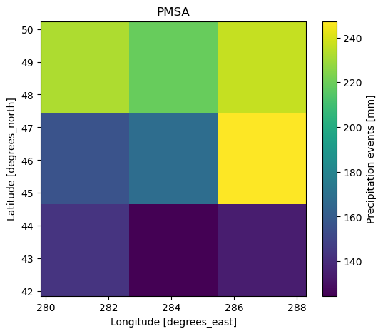
9.2.4. PMSA estimation
The PMSA is the highest total among all winters defined.
[27]:
pmsa = snow_sum.resample(time="YS-JUL").sum(dim="time").max(dim="time")
pmsa
[27]:
<xarray.DataArray 'non_max_snow_events' (window: 1, y: 3, x: 3)> Size: 72B
dask.array<_nanmax_skip-aggregate, shape=(1, 3, 3), dtype=float64, chunksize=(1, 3, 3), chunktype=numpy.ndarray>
Coordinates:
  * window    (window) int64 8B 1
  * y         (y) float64 24B 43.25 46.04 48.84
  * x         (x) float64 24B 281.2 284.1 286.9
    height    float64 8B 2.0
quantile float64 8B 0.99[28]:
plt.subplots(1, 1, figsize=[6, 5])
ax = plt.subplot(1, 1, 1)
pmsa.sel(window=1).plot()
plt.title("PMSA")
/home/docs/checkouts/readthedocs.org/user_builds/xhydro/conda/stable/lib/python3.14/site-packages/dask/_task_spec.py:768: RuntimeWarning: divide by zero encountered in divide
/home/docs/checkouts/readthedocs.org/user_builds/xhydro/conda/stable/lib/python3.14/site-packages/dask/_task_spec.py:768: RuntimeWarning: invalid value encountered in divide
[28]:
Text(0.5, 1.0, 'PMSA')