8. Analyse des valeurs extrêmes utilisant Extremes.jl
Ce module fournit une interface facile à utiliser pour le package Extremes.jl en Julia, permettant une intégration fluide avec xarray pour l’analyse des valeurs extrêmes. Cependant, veuillez noter que juliacall n’est pas installé par défaut lors de l’installation de xHydro. Consultez la page d’installation pour des instructions.
Le package Extremes.jl est spécialement conçu pour l’analyse des valeurs extrêmes et offre une variété de fonctionnalités puissantes :
Méthodes des maxima par blocs et de dépassements de seuil, y compris des distributions populaires telles que
genextreme,gumbel_retgenpareto.Techniques flexibles d’estimation des paramètres, prenant en charge des méthodes telles que
Probability-Weighted Moments (PWM),Maximum Likelihood Estimation (MLE), etBayesian Estimation.Compatibilité avec les modèles stationnaires et non stationnaires pour une modélisation flexible des événements extrêmes futurs.
Estimation du niveau de retour pour quantifier le risque d’événements extrêmes sur différentes périodes de retour.
Pour plus d’informations sur le package Extremes.jl, consultez les ressources suivantes :
[1]:
import os

os.environ["PYTHON_JULIACALL_AUTOLOAD_IPYTHON_EXTENSION"] = (
    "no"  # To prevent random crashes with GitHub's testing interface
)

import matplotlib.pyplot as plt
import numpy as np
import pandas as pd
import pooch
from IPython.display import clear_output

import xhydro.extreme_value_analysis as xhe
from xhydro.testing.helpers import deveraux

clear_output(wait=False)
8.1. Acquisition des données
Cet exemple utilisera les données du modèle climatique GFDL-ESM4.1 pour démontrer la non-stationnarité. Le jeu de données inclut des données de précipitations annuelles totales de 1955 à 2100, couvrant 97 stations virtuelles à travers la province de Québec. Pour plus d’informations sur comment accéder aux données de précipitations ou effectuer des maxima par blocs, consultez le Notebook Analyses fréquentielles locales.
[2]:
file = deveraux().fetch("extreme_value_analysis/NOAA_GFDL_ESM4.zip", pooch.Unzip())
[3]:
df = pd.read_csv(file[0], parse_dates=[0])[
    ["time", "station_num", "station_name", "total_precip"]
]
# That dataset is a CSV file, so we need to format it
ds = df.to_xarray()
ds = ds.set_coords(["time", "station_num", "station_name"])
ds = ds.set_index(index=["station_num", "time"])
ds = ds.unstack("index")
ds["total_precip"].attrs["units"] = "mm y-1"

# Take a subset for the example
ds = ds.isel(station_num=slice(0, 5))
ds
[3]:
<xarray.Dataset> Size: 13kB
Dimensions:       (station_num: 5, time: 146)
Coordinates:
  * station_num   (station_num) int64 40B 1001 1004 1008 1009 1012
  * time          (time) datetime64[ns] 1kB 1955-01-01 1956-01-01 ... 2100-01-01
    station_name  (station_num, time) object 6kB 'Dozois' ... 'Lac St-Francois'
Data variables: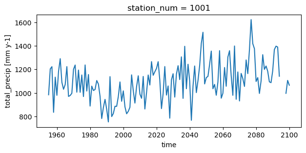
total_precip (station_num, time) float64 6kB 983.6 1.204e+03 ... 1.065e+03[4]:
plt.figure(figsize=[7, 3])
ds.isel(station_num=0).total_precip.plot()
[4]:
[<matplotlib.lines.Line2D at 0x7fa05413bb30>]
ATTENTION
Actuellement, il n’est pas possible de fournir à Extremes.jl un ensemble prédéfini de paramètres pour calculer directement les périodes de retour. Jusqu’à ce que cette fonctionnalité soit implémentée dans xHydro ou Extremes.jl, les fonctions .fit() et .return_level() doivent être considérées comme indépendantes. Plus précisément, la fonction .return_level() estimera d’abord les paramètres de la distribution avant de calculer les niveaux de retour.
8.2. Estimation des paramètres
La fonction xhydro.extreme_value_analysis.fit sert d’interface entre xHydro et le package Extremes.jl. La plupart des arguments sont identiques à ceux utilisés dans la fonction xhydro.frequency_analysis.local.fit. Les noms des distributions statistiques ont été alignés avec ceux de SciPy. Voici quelques différences principales :
Méthode bayésienne (
BAYES) : Lors de l’utilisation de la méthodeBAYES, vous pouvez spécifier deux paramètres supplémentaires :niter: Nombre d’itérations pour l’algorithme d’inférence bayésienne.warmup: Nombre d’itérations de préchauffage pour l’inférence bayésienne.
Intervalles de confiance : Un ajout important à cette fonction est le paramètre
confidence_level, qui simplifie le processus d’obtention de l’intervalle de confiance par rapport aux autres options disponibles dansxHydro, comme expliqué dans les autres Notebooks d’analyse fréquentielle.
Dans cet exemple, nous estimerons une distribution des Valeurs Extrêmes Généralisées (GEV) (genextreme) en utilisant la méthode des Moments Pondérés par la Probabilité (PWM). De plus, nous calculerons et renverrons les intervalles de confiance à 95 % pour les paramètres estimés.
[5]:
help(xhe.fit)
Help on function fit in module xhydro.extreme_value_analysis.parameterestimation:

fit(ds: 'xr.Dataset', locationcov: 'list[str] | None' = None, scalecov: 'list[str] | None' = None, shapecov: 'list[str] | None' = None, variables: 'list[str] | None' = None, dist: 'str | scipy.stats.rv_continuous' = 'genextreme', method: 'str' = 'ML', dim: 'str' = 'time', confidence_level: 'float' = 0.95, niter: 'int' = 5000, warmup: 'int' = 2000) -> 'xr.Dataset'
    Fit an array to a univariate distribution along a given dimension.

    Parameters
    ----------
    ds : xr.DataSet
        Xarray Dataset containing the data to be fitted.
    locationcov : list[str]
        List of names of the covariates for the location parameter.
    scalecov : list[str]
        List of names of the covariates for the scale parameter.
    shapecov : list[str]
        List of names of the covariates for the shape parameter.
    variables : list[str]
        List of variables to be fitted.
    dist : str or rv_continuous distribution object
        Name of the univariate distribution or the distribution object itself.
        Supported distributions are genextreme, gumbel_r, genpareto.
    method : {"ML", "PWM", "BAYES}
        Fitting method, either maximum likelihood (ML), probability weighted moments (PWM) or bayesian (BAYES).
    dim : str
        Specifies the dimension along which the fit will be performed (default: "time").
    confidence_level : float
        The confidence level for the confidence interval of each parameter.
    niter : int
        The number of iterations of the bayesian inference algorithm for parameter estimation (default: 5000).
    warmup : int
        The number of warmup iterations of the bayesian inference algorithm for parameter estimation (default: 2000).

    Returns
    -------
    xr.Dataset
        Dataset of fitted distribution parameters and confidence interval values.

    Notes
    -----
    Coordinates for which all values are NaNs will be dropped before fitting the distribution. If the array still
    contains NaNs or has less valid values than the number of parameters for that distribution,
    the distribution parameters will be returned as NaNs.
[6]:
fit_stationary = xhe.fit(
    ds,
    dist="genextreme",
    method="PWM",
    variables=["total_precip"],
    confidence_level=0.95,
)
fit_stationary
[6]:
<xarray.Dataset> Size: 460B
Dimensions:             (station_num: 5, dparams: 3)
Coordinates:
  * station_num         (station_num) int64 40B 1001 1004 1008 1009 1012
  * dparams             (dparams) <U5 60B 'shape' 'loc' 'scale'
Data variables:
    total_precip        (station_num, dparams) float64 120B 0.2012 ... 155.8
    total_precip_lower  (station_num, dparams) float64 120B 0.08579 ... 135.3
total_precip_upper (station_num, dparams) float64 120B 0.3243 ... 174.18.3. Périodes de retour
Comme mentionné dans l’avertissement ci-dessus, la fonction xhydro.extreme_value_analysis.return_level ne peut pas accepter de paramètres prédéfinis et Extremes.jl doit les calculer en interne. Par conséquent, avec l’inclusion de l’argument return_period, tous les paramètres de la fonction restent les mêmes.
Dans cet exemple, nous estimerons une distribution de Gumbel (gumbel_r) en utilisant la méthode du Maximum de Vraisemblance (ML). De plus, nous calculerons et renverrons les intervalles de confiance à 95 % pour les paramètres estimés.
[7]:
help(xhe.return_level)
Help on function return_level in module xhydro.extreme_value_analysis.parameterestimation:

return_level(ds: 'xr.Dataset', locationcov: 'list[str] | None' = None, scalecov: 'list[str] | None' = None, shapecov: 'list[str] | None' = None, variables: 'list[str] | None' = None, dist: 'str | scipy.stats.rv_continuous' = 'genextreme', method: 'str' = 'ML', dim: 'str' = 'time', confidence_level: 'float' = 0.95, return_period: 'float' = 100, niter: 'int' = 5000, warmup: 'int' = 2000, threshold_pareto: 'float | None' = None, nobs_pareto: 'int | None' = None, nobsperblock_pareto: 'int | None' = None) -> 'xr.Dataset'
    Compute the return level associated with a return period based on a given distribution.

    Parameters
    ----------
    ds : xr.DataSet
        Xarray Dataset containing the data for return level calculations.
    locationcov : list[str]
        List of names of the covariates for the location parameter.
    scalecov : list[str]
        List of names of the covariates for the scale parameter.
    shapecov : list[str]
        List of names of the covariates for the shape parameter.
    variables : list[str]
        List of variables to be fitted.
    dist : str or rv_continuous distribution object
        Name of the univariate distribution or the distribution object itself.
        Supported distributions are genextreme, gumbel_r, genpareto.
    method : {"ML", "PWM", "BAYES}
        Fitting method, either maximum likelihood (ML), probability weighted moments (PWM) or bayesian (BAYES).
    dim : str
        Specifies the dimension along which the fit will be performed (default: "time").
    confidence_level : float
        The confidence level for the confidence interval of each parameter.
    return_period : float
        Return period used to compute the return level.
    niter : int
        The number of iterations of the bayesian inference algorithm for parameter estimation (default: 5000).
    warmup : int
        The number of warmup iterations of the bayesian inference algorithm for parameter estimation (default: 2000).
    threshold_pareto : float
        The value above which the Pareto distribution is applied.
    nobs_pareto : int
        The total number of observations used when applying the Pareto distribution.
    nobsperblock_pareto : int
        The number of observations per block when applying the Pareto distribution.

    Returns
    -------
    xr.Dataset
        Dataset of with the return level and the confidence interval values.

    Notes
    -----
    Coordinates for which all values are NaNs will be dropped before fitting the distribution. If the array still
    contains NaNs or has less valid values than the number of parameters for that distribution,
    the distribution parameters will be returned as NaNs.
[8]:
rtnlv_stationary = xhe.return_level(
    ds,
    dist="gumbel_r",
    method="ML",
    variables=["total_precip"],
    confidence_level=0.95,
    return_period=100,
)
rtnlv_stationary
[8]:
<xarray.Dataset> Size: 168B
Dimensions:             (station_num: 5, return_period: 1)
Coordinates:
  * station_num         (station_num) int64 40B 1001 1004 1008 1009 1012
  * return_period       (return_period) int64 8B 100
Data variables:
    total_precip        (station_num, return_period) float64 40B 1.704e+03 .....
    total_precip_lower  (station_num, return_period) float64 40B 1.609e+03 .....
total_precip_upper (station_num, return_period) float64 40B 1.8e+03 ... ...8.4. Modèle non stationnaire
Jusqu’à présent, nous avons ignoré trois arguments supplémentaires—locationcov, scalecov et shapecov—qui acceptent des noms de variables. Ces arguments vous permettent d’introduire un aspect non linéaire dans le modèle statistique. Dans les modèles non stationnaires, des variables explicatives (covariables) peuvent être utilisées pour capturer les changements dans les paramètres du modèle au fil du temps ou selon différentes conditions. Ces covariables peuvent représenter des facteurs tels que le temps, la localisation géographique, l’augmentation de la température mondiale ou les concentrations de CO2, ou toute autre variable qui pourrait influencer les paramètres de la distribution.
Notez également que la méthode PWM ne peut pas être utilisée avec des modèles non stationnaires.
Pour cet exemple, nous allons simplifier les choses et supposer que le paramètre de localisation varie de manière linéaire avec l’année. Pour ce faire, nous devrons ajouter une nouvelle variable contenant l’année à notre jeu de données et fournir ensuite cette variable à l’argument locationcov.
[9]:
ds["year"] = ds.time.dt.year.broadcast_like(ds["total_precip"])
ds
[9]:
<xarray.Dataset> Size: 19kB
Dimensions:       (station_num: 5, time: 146)
Coordinates:
  * station_num   (station_num) int64 40B 1001 1004 1008 1009 1012
  * time          (time) datetime64[ns] 1kB 1955-01-01 1956-01-01 ... 2100-01-01
    station_name  (station_num, time) object 6kB 'Dozois' ... 'Lac St-Francois'
Data variables:
    total_precip  (station_num, time) float64 6kB 983.6 1.204e+03 ... 1.065e+03
year (station_num, time) int64 6kB 1955 1956 1957 ... 2099 2100Dans le cas de la fonction .fit(), l’ajout d’une covariable introduira une nouvelle entrée sous la dimension dparams. Pour cet exemple, elle a créé une nouvelle entrée appelée loc_year_covariate sous la dimension dparams.
[10]:
fit_non_stationary = xhe.fit(
    ds,
    dist="genextreme",
    method="ML",
    variables=["total_precip"],
    locationcov=["year"],
    confidence_level=0.95,
)
fit_non_stationary
[10]:
<xarray.Dataset> Size: 808B
Dimensions:             (station_num: 5, dparams: 4)
Coordinates:
  * station_num         (station_num) int64 40B 1001 1004 1008 1009 1012
  * dparams             (dparams) <U18 288B 'shape' 'loc' ... 'scale'
Data variables:
    total_precip        (station_num, dparams) float64 160B 0.2051 ... 144.3
    total_precip_lower  (station_num, dparams) float64 160B 0.1022 ... 127.0
total_precip_upper (station_num, dparams) float64 160B 0.308 ... 164.0Dans le cas de la fonction .return_level(), l’ajout d’une covariable préserve les dimensions d’origine, y compris la dimension le long de laquelle le return_level est calculé (par exemple, le temps).
[11]:
rtnlv_non_stationary = xhe.return_level(
    ds,
    dist="gumbel_r",
    method="ML",
    dim="time",
    variables=["total_precip"],
    locationcov=["year"],
    confidence_level=0.95,
    return_period=100,
)

rtnlv_non_stationary
[11]:
<xarray.Dataset> Size: 25kB
Dimensions:             (station_num: 5, time: 146, return_period: 1)
Coordinates:
  * station_num         (station_num) int64 40B 1001 1004 1008 1009 1012
  * time                (time) datetime64[ns] 1kB 1955-01-01 ... 2100-01-01
    station_name        (station_num, time) object 6kB 'Dozois' ... 'Lac St-F...
  * return_period       (return_period) int64 8B 100
Data variables:
    total_precip        (station_num, time) float64 6kB 1.557e+03 ... 1.771e+03
    total_precip_lower  (station_num, time) float64 6kB 1.457e+03 ... 1.672e+03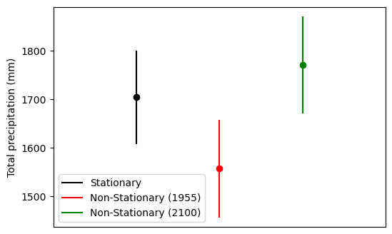
total_precip_upper (station_num, time) float64 6kB 1.656e+03 ... 1.87e+038.4.1. Comparaison des périodes de retour en utilisant les modèles stationnaire et non stationnaire
[12]:
import matplotlib.pyplot as plt
import numpy as np

fig, ax = plt.subplots()
fig.set_figheight(4)
fig.set_figwidth(6)

# Stationary fit
plt.plot(
    np.array([1, 1]),
    np.array(
        [
            rtnlv_stationary.total_precip_lower.isel(station_num=0),
            rtnlv_stationary.total_precip_upper.isel(station_num=0),
        ]
    ),
    "black",
    label="Stationary",
)
plt.scatter(
    np.array([1]),
    np.array([rtnlv_stationary.total_precip.isel(station_num=0)]),
    c="black",
)

plt.plot(
    np.array([2, 2]),
    np.array(
        [
            rtnlv_non_stationary.total_precip_lower.isel(station_num=0, time=0),
            rtnlv_non_stationary.total_precip_upper.isel(station_num=0, time=0),
        ]
    ),
    "red",
    label="Non-Stationary (1955)",
)
plt.scatter(
    np.array([2]),
    np.array([rtnlv_non_stationary.total_precip.isel(station_num=0, time=0)]),
    c="red",
)

plt.plot(
    np.array([3, 3]),
    np.array(
        [
            rtnlv_non_stationary.total_precip_lower.isel(station_num=0, time=-1),
            rtnlv_non_stationary.total_precip_upper.isel(station_num=0, time=-1),
        ]
    ),
    "green",
    label="Non-Stationary (2100)",
)
plt.scatter(
    np.array([3]),
    np.array([rtnlv_non_stationary.total_precip.isel(station_num=0, time=-1)]),
    c="green",
)

plt.xlim([0, 4])
plt.xticks([])
plt.ylabel("Total precipitation (mm)")
ax.legend()
[12]:
<matplotlib.legend.Legend at 0x7f9f63a61340>
8.5. Travailler avec dask.array
Actuellement, l’interaction Python-Julia n’est pas sûre pour les threads. Pour atténuer les problèmes potentiels, il est recommandé d’utiliser l’option dask.scheduler="processes" lors du calcul des résultats. Cela garantit que les tâches sont exécutées dans des processus Python séparés, offrant ainsi une meilleure isolation et évitant les conflits liés aux threads.
[ ]:
ds_c = ds.chunk({"time": -1, "station_num": 1})

fit_stationary_c = xhe.fit(
    ds_c,
    dist="genextreme",
    method="ml",
    variables=["total_precip"],
    confidence_level=0.95,
)
fit_stationary_c = fit_stationary_c.compute(scheduler="processes")
clear_output(wait=False)
[14]:
fit_stationary_c
[14]:
<xarray.Dataset> Size: 460B
Dimensions:             (station_num: 5, dparams: 3)
Coordinates:
  * station_num         (station_num) int64 40B 1001 1004 1008 1009 1012
  * dparams             (dparams) <U5 60B 'shape' 'loc' 'scale'
Data variables:
    total_precip        (station_num, dparams) float64 120B dask.array<chunksize=(1, 3), meta=np.ndarray>
    total_precip_lower  (station_num, dparams) float64 120B dask.array<chunksize=(1, 3), meta=np.ndarray>
    total_precip_upper  (station_num, dparams) float64 120B dask.array<chunksize=(1, 3), meta=np.ndarray>